Type IMG data tree entries: 2-D Images
An IMG data tree entry is created whan a 2D diffraction image is imported into a GSAS-II project. Note that unlike every other type of entry in the GSAS-II data tree, images are not self-contained. The actual contents of the image is read from the original file whenever the image is needed, but all other settings utilized in image processing other than the image itself are stored inside the project. If the .gpx file is moved to another computer, if it contains images, the image files must also be moved.
A IMG data tree entry is always accompanied by four child tree entries, labeled Comments, Image Controls, Masks and Stress/Strain. There is also some information in the parent IMG entry.
When a 2D diffraction image (prefix IMG) or one of its children is selected from the data tree, the image is displayed as a color contoured picture. At a minimum, a small 'X' shows the currently defined location of the incident beam on the image plane (NB: it could be off to one side or the other depending on detector location, or even outside of the image). Optionally, the integration limits are shown as an interior arc, an outer arc and green (beginning \(2\theta\) limit) and red (ending \(2\theta\) limit) as well as “cake” section limits (dashed lines) connecting the two. These are set in Image Controls. There may be a frame mask (green) that encloses the area used for subsequent integration or other analysis. Red outlines and pixels indicated selected areas/pixels that are excluded (masked) from further use; the settings for these are found in Masks.
Parent IMG data tree entry
The data window for the main IMG data tree entry shows some controls, most of which are rarely modified (e.g., pixel dimensions) and are usually obtained via the image importer from either the image header or a metadata file associated with the image. It is the user's/instrument scientist's responsibility to ensure the accuracy of these values. When they are wrong, the image cannot be used.
What can I do here?
-
A number of calibration values are shown for the placement and dimensions of the detector. They can be changed here. (Caution: you do need to know what their true value is; you do not want to invalidate data by incorrectly changing these values.)
-
Polarization: you can determine the x-ray beam polarization for your detector. This requires an image with scattering from a purely isotropic amorphous sample (a glass slide mounted perpendicular to the incident beam is recommended) with the detector close to the sample so that the scattering angle at the edge of the detector is at least 35° \(2\theta\); better is > 40° \(2\theta\). A frame mask is recommended to remove detector edge effects. The image should be as free as possible (except for beam stop) from shadows and obstructions and normal to the incident beam. The detector orientation should have been previously calibrated with a known reference material (e.g., LaB6 or Si). Use the Calibrate? button to start the Polarization process, as below.
- Calibrate? (Polarization) - This begins the calibration procedure (Von Dreele & Xi, 2021) for the x-ray beam polarization, which integrates a 4° \(2\theta\) wide ring sampling area with and without an arc mask positioned about 90° azimuth (top of image) with selected polarization values. The integrations match with the correct polarization value. You will be asked for a \(2\theta\) position for the sampling mask; choose a value at least 2° \(2\theta\) less than the maximum \(2\theta\) seen for all edges inside the frame mask. The process takes about 5 min to complete, so be patient.
Comments
This window shows whatever comment lines found in a “metadata” file when the image data file was read by GSAS-II. If you are lucky, there will be useful information here (e.g., sample name, date collected, wavelength used, etc.). With some types of files, this window will be blank. The text is read-only. It will be transferred over to diffraction patterns when the image is integrated and can be used to set parametric values (in Sample Parameters) associated with the diffraction pattern.
What can I do here?
Nothing.
Image Controls
The image controls data window displays a number of settings and options that include calibration values needed to convert pixel locations to two-theta and azimuth, values used to integrate the image, settings that adjustment the image, settings used when performing image calibration and sample setting angles.
What can I do here?
- Perform image calibration with data from a standard
- Create a gain map (requires multiple images)
- Integrate images
Window organization
The window used for Image Controls contains a large number of settings and controls, as shown below. The sections of the window are outlined below with colored boxes and labeled that are described further, also below.
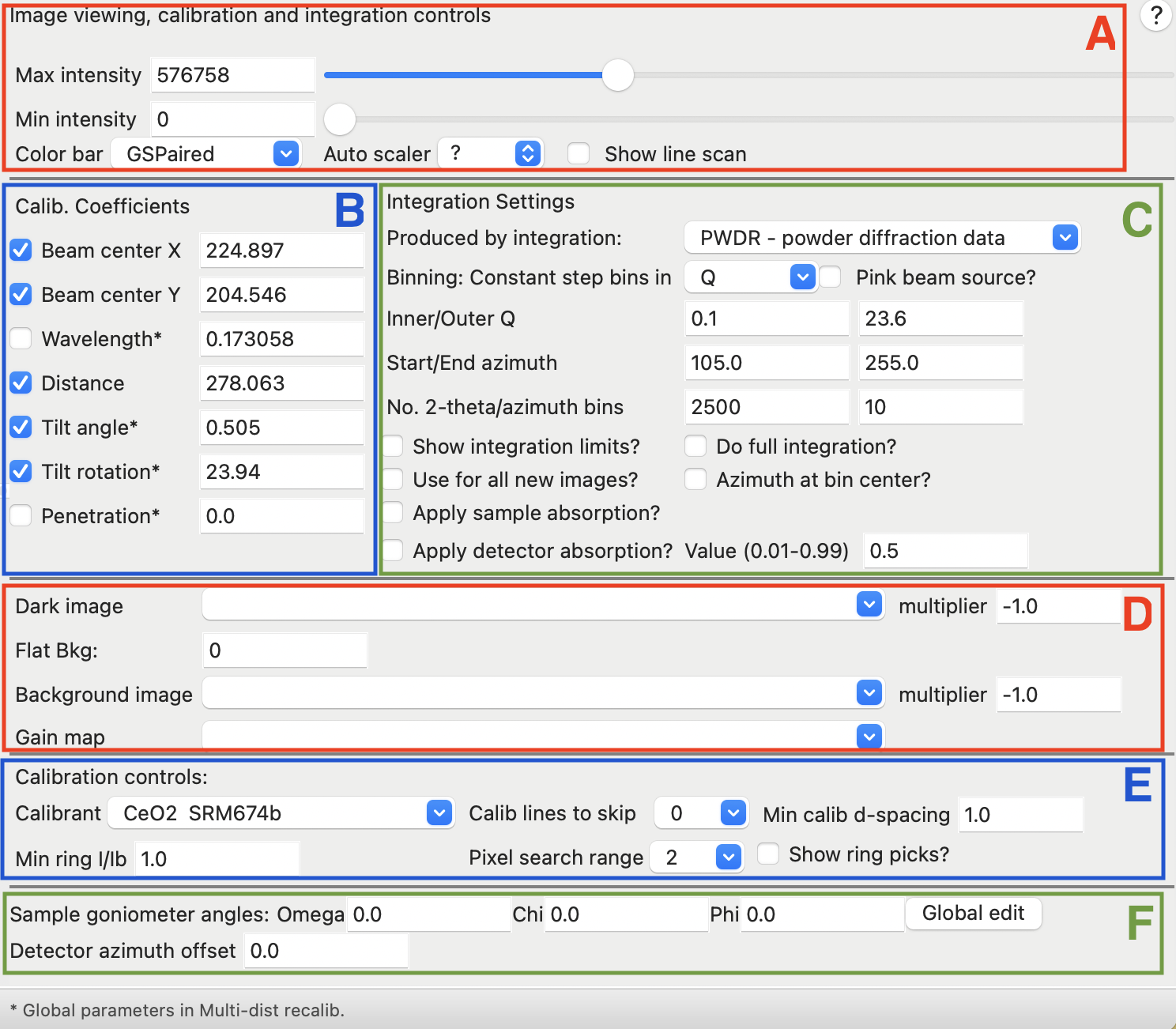
- A. The Image controls section at the top has controls that determine how the image is displayed. These settings do not affect computations from the image.
- B. The Calibration coefficients have the results from an image calibration and are used to determine the \(2\theta\) value for each pixel in the image.
- C. The Integration coefficients determine how image integration is performed. Show integration limits will show lines on the image, but does not change the integration results.
- D. Image corrections: It is possible to subtract images from the current image to account for pixels that provide non-zero results even when not illuminated (Dark image); or a constant value that is subtracted from all pixels (Flat Bkg), as well as subtract an image with scattering from the instrument or sample container (Background image). It is also possible to adjust for pixel-by-pixel detector response with a gain map.
- E. The Calibration controls determine the process used to search for diffraction rings when the detector calibration is used. The "Show ring picks" check button determines if the located ring positions are displayed, but does not affect the computation.
- F. The Sample goniometer angles reflect positioning of a sample. They are not used for calibration, but will be transferred to powder patterns generated from the image during image integration. The Global edit button provides a single window where setting angles for all images can be changed.
Menu commands
Three sets of menu commands are associated with the Image Controls tree item. The first, Calibration, provides commands to perform calibration from an image (where the calibration values are fitted from a diffraction pattern image taken with a calibrant).
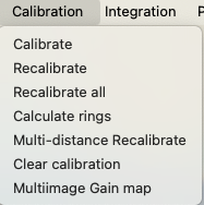 * Calibrate: The calibrate command will expect you to have already set a calibrant and as well as any other settings in the Calibration controls and then to click on several points for the first diffraction ring with the left mouse button. Then click on the right mouse button to begin the calibration process, which will search for the location of additonal rings.
* Recalibrate: Repeats the calibration process using the previously-located position for the first ring and current image settings.
* Recalibrate all: Repeats the calibration process using the previously-located position for the first ring and current image settings, but for a series of selected images.
* Calculate rings: Computes and displays the ring positions from the calibration settings. Does not change any values.
* Multi-distance Recalibrate: Performs a calibration on a series of images that have different distance placements. The tilt angle, the tilt rotation, the penetration and the wavelength, will be required to be the same for all included images, if refined. The beam center X & Y values are independent for each image. This command can operate in two modes: If any of the detector distance settings are set to be refined, then those distances are optimized individually (the wavelength cannot be refined in this case). If none of the distances are set to be refined, then a overall offset for all detectors is fit. The wavelength parameter will also be refined if the refine flag is on for the first image.
* Clear calibration: Deletes previous ring pick information from the current image
* Calibrate: The calibrate command will expect you to have already set a calibrant and as well as any other settings in the Calibration controls and then to click on several points for the first diffraction ring with the left mouse button. Then click on the right mouse button to begin the calibration process, which will search for the location of additonal rings.
* Recalibrate: Repeats the calibration process using the previously-located position for the first ring and current image settings.
* Recalibrate all: Repeats the calibration process using the previously-located position for the first ring and current image settings, but for a series of selected images.
* Calculate rings: Computes and displays the ring positions from the calibration settings. Does not change any values.
* Multi-distance Recalibrate: Performs a calibration on a series of images that have different distance placements. The tilt angle, the tilt rotation, the penetration and the wavelength, will be required to be the same for all included images, if refined. The beam center X & Y values are independent for each image. This command can operate in two modes: If any of the detector distance settings are set to be refined, then those distances are optimized individually (the wavelength cannot be refined in this case). If none of the distances are set to be refined, then a overall offset for all detectors is fit. The wavelength parameter will also be refined if the refine flag is on for the first image.
* Clear calibration: Deletes previous ring pick information from the current image
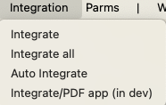
The Integration menu provides the ability to radially integrate an image to provide one or more powder diffraction patterns (requires that calibration parameters must be set first.)
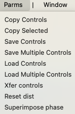
Finally, the Parms menu has commands allow the values on the window to be saved to a file, read from a file or copied to other images. The "Xfer controls" menu command differs from the "Copy Controls" command in that integration range for the current image is scaled when applied for other images based on the detector distances.
Calibration parameters definitions
The detector coordinate system has x horizontal and y vertical with (0,0) located at the lower left, looking from the sample position. The z axis is defined as z = x \(\times\) y, which points from the detector towards the sample. When a detector is rotated from this position, the detector azimuthal offset describes the angle applied to rotate the detector clockwise (as viewed from the sample position) from the orientation with x horizontal and y vertical. The beam center position in GSAS-II is in mm, measured from the bottom left corner of the detector.
Comparison to other software
Note that calibration parameters used in GSAS-II are closely related to those used by the pyFAI and Fit2D programs, but add 90 to the GSAS-II tilt plane rotation (labeled as "Rotation" in GSAS-II) to obtain the pyFAI value. The beam center location in pyFAI is defined the the same way as in GSAS-II, except that in pyFAI the units are pixels rather than in mm.
and
For Fit2D, the center is also in mm, but measured from the bottom left, so
and
where \(Y_{max}\) is the detector size in pixels and \(size_X\) and \(size_Y\) are the pixel size in mm along the appropriate direction.
Masks
The information on the Masks window are used to determine what parts of an image will not be included in the integration, typically used due to detector irregularities, shadows of the beam stop, single-crystal peaks from a mounting, cosmic rays, etc.
Note that the top section of the window repeats some of the display controls from the Image Controls window. These are duplicated so that the image can be viewed under different conditions without needing to switch between the different data items.
Sections of the image may removed from integration by one or all of the following options.
-
The Upper/Lower Thresholds designate the allowed values for pixels to be considered valid. Typically detectors will set pixels that are in margins between segments etc. and are not in use to have negative intensity values, so a threshold of 0 causes these pixels to be ignored. Likewise, malfunctioning pixels or those picking up anomalous signals, such as cosmic rays, may have exceptionally high intensity values that should also be ignored.
-
Pixel masking excludes individual pixels that have intensities that are significantly higher or lower than the median intensity across single \(2\theta\) value. The controls for the pixel mask search determine the threshold for exclusion, which is expressed as a multiple of the median-based standard deviation for the \(2\theta\) ring; the minimum and maximum \(2\theta\) value to be used in the search; and if the search should replace any previous pixel map search(es) or should be added to the previous pixel mask search. This latter control, when "Clear..." is turned off, allows the sensitivity for exclusion to be varied for different \(2\theta\) ranges. Finally, a button allows a previous pixel mask to be cleared.
-
Specific geometrical regions of the detector can be designated to be ignored using menu commands or with keyboard/mouse shortcuts.
There are five types of geometrical masks:
- Spot masks: exclude a circle with a selected center and diameter in image coordinates (mm).
- Ring masks: excludes a specific Bragg reflection (a ring placed relative to the image center). The location and thickness of the ring are specified in degrees 2-theta.
- Arc masks: exclude a section of a Bragg reflection, similar to a ring mask, except that in addition to the location and thickness of the ring, the mask has a starting and ending azimuthal angle.
- Polygon masks: exclude an arbitrary region created by line segments joining a series of points specified in image coordinates (mm). Pixels inside the polygon mask are not used for integration.
- Frame mask: excludes an arbitrary region created by line segments joining a series of points specified in image coordinates (mm). Typically, a point is placed near each corner of the image. Only pixels inside the frame mask are used for integration. Only one frame mask can be defined.
What can I do here?
Masks of each type are created using the appropriate menu commands and then clicking as described in the section on "What can I do with the plot?" below, or by using keyboard shortcuts, also described in that section.
What is plotted here?
The image is shown, as described above. Note that the frame mask, if defined, is displayed in green, while the other types of masks are shown in red.
What can I do with the plot?
There are menu commands to create masks as well as keyboard shortcuts. If a menu command is used, then use left and right mouse clicks as described below. Note that on a Mac with a one-button mouse, some alternate actions must be used.
-
Spot masks: excludes inside a circular region of the image.
-
Create Spot masks after a menu command by clicking on the location on the image that should be masked. There are also two ways to create spot masks with the keyboard:
- Press the 's' key and then left-click successively on multiple locations for spot masks. Press the 's' key again or right-click to stop adding spot masks.
- Alternately, move the mouse to the position for a new spot mask and press the 't' key. (Note that this can be used while the plot is in Zoom or Pan mode.)
The default size for newly-created spot masks is determined by the
Spot_mask_diameterconfiguration variable or 1.0 mm, if not specified. -
Edit Spot mask location by left-clicking inside or on the edge the of the mask and then drag the spot mask to a new location.
-
Edit Spot mask radius by right-clicking inside the mask and then dragging to change the mask size.
-
-
Ring masks: excludes inside a ring of selected width that follows constant \(2\theta\) as determined by the calibration (e.g. a Bragg diffraction ring).
-
Create Ring masks with a menu command and then by left-clicking on the mask center; Or, by pressing the 'r' key and then left-clicking. (Right-click to cancel.)
The default thickness for newly-created ring masks is determined by the
Ring_mask_thicknessconfiguration variable or 0.1 degrees (\(2\theta\)) if not specified. -
Edit Ring mask location by left-clicking on either the inner or outer circle and drag the circle to the new radius.
-
Edit Ring mask thickness by right-clicking either on the inner or outer circle and drag the the circle change spacing between the inner and outer circle.
-
-
Arc masks: excludes inside an arc of constant \(2\theta\), similar to a ring mask, except that in addition to the location and thickness of the ring, the mask has a starting and ending azimuthal angle.
-
Create Arc masks with a menu command and then by left-clicking on at the mask center; Or, by pressing the 'a' key and then left-clicking. (Right-click to cancel.)
The default size for newly-created ring masks is determined by configuration variables:
- thickness:
Ring_mask_thickness(0.1 degrees \(2\theta\) if not specified) and - azimuthal range:
Arc_mask_azimuth(10.0 degrees if not specified.)
- thickness:
-
Edit Arc mask location by left-clicking on either the inner or outer circle and drag the circle to the new radius. Alternately, left-click on the upper or lower arc limit (the straight lines) and drag them to rotate the center of the arc azimuthal range to a new position.
-
Edit Arc mask thickness or range by right-clicking either on the inner or outer circle and drag the the circle change spacing between the inner and outer circle. Alternately, right-click on the upper or lower arc limit (the straight lines) and drag them to change the arc azimuthal range.
-
-
Polygon masks: excludes inside an arbitrary region created by line segments joining a series of points specified in image coordinates (mm). Pixels inside the polygon mask are not used for integration.
-
Create Polygon masks with a menu command and then by left-clicking successively on the vertices of the polygon shape surrounding pixels to be excluded. After the last point is defined, right-click anywhere to close the mask. Alternately, press the 'p' key and then left-click, as before, to define the mask and right-click anywhere to close the mask.
-
Edit Polygon mask by left-clicking on any point at a vertex in the polygon mask and drag that point to a new position. If the vertex is dragged to the same position as any other vertex in the mask the dragged point is deleted.
-
Add a point to Polygon mask by right-clicking on any vertex and dragging. A new point is added to the mask immediately after the selected point at the position where the mouse is released.
-
-
Frame mask: excludes outside an arbitrary region created by line segments joining a series of points specified in image coordinates (mm). Typically, a point is placed near each corner of the image. Only pixels inside the frame mask are used for integration. Only one frame mask can be defined.
-
Create a Frame mask with a menu command and then by left-clicking successively on the vertices of a polygon. After the last point is defined, right-click anywhere to close the frame mask. Alternately, press the 'f' key and then left-click, as before, to define the mask and right-click anywhere to close the mask. Note that if a Frame mask already exists, using the 'f' key or the "Create Frame" menu item causes the existing frame mask to be deleted.
-
Edit the Frame mask by left-clicking on any point at a vertex in the frame mask and drag that point to a new position. If the vertex is dragged to the same position as any other vertex in the mask the dragged point is deleted.
-
Add a point to the Frame mask by right-clicking on any vertex and dragging. A new point is added to the mask immediately after the selected point at the position where the mouse is released.
-
-
Pixel mask: excludes individual pixels that are found in a pixel mask search, which looks for pixels that have intensities that are higher or lower by a threshhold than the median intensity for all pixels in a ring with the same two-theta value. By default this mask contains no pixels, but pixels are added using a search.
- Search to add to the pixel mask using either the Operations->"Pixel mask search" or the Operations->"Multi-IMG pixel mask search" menu commands. This searches for pixels that have intensities that are significantly higher or lower than the median intensity for all pixels in a ring having the same two-theta value. The threshold for exclusion is determined by the standard deviation for the pixels in the ring multiplied by a user-supplied value.
Stress/Strain
This allows one to evaluate strain typically induced by a pure axial load (e.g. no shear) on a polycrystalline sample (e.g. a steel bar). This strain will distort the Bragg diffraction rings seen by the 2D detector. This follows the method of He & Smith (Baoping Bob He & Kingsley Smith, (1997). Adv. in X-Ray Anal. 41, 501.) to determine the 3 unique terms of the axial strain tensor. One can examine the results as a series of diffraction line d-spacings vs azimuth angle; if no strain, these are straight, otherwise they will show a single sinusoidal variation with maxima at the maximum strain direction (90° & 270°) for a tension load. The signs are reversed for a compression load. One can also examine the local intensity variation as multiples of a random distribution (MRD) due to texture. Before embarking on this analysis be sure that your detector is carefully calibrated for orientation and position; you are looking for very slight variations in ring shape which may be biased by inadequate detector calibration. Commonly, the calibrant (typically \(\rm CeO_2\)) is painted on one sample surface (be sure to note if in front or back of sample!) and the sample ½ thickness is used in the Sample delta-z box (significant only for residual stress analysis).
What can I do here?
Menu Operations -
- Append d-zero – this adds a d-spacing value to the stress strain ring list; this also can be done by picking a ring from the plot.
- Fit stress/strain – this fits the three unique axial strain tensor elements (ε11, ε22 & ε12) for each ring to the local ring maxima at 1 mm intervals about each ring. Results display on console and table. The fitted d-zero is calculated from the mean d-spacings found for the ring & given as d-zero ave and can be compared to the d-zero value for any residual stress/strain.
- Plot intensity distribution – this makes an MRD plot with azimuth for each ring.
- Save intensity distribution – this saves the intensity distribution curves as a simple text file
- Update d-zero – this updates the d-zero values with the d-zero ave ones thus removing any effect of residual stress/strain.
- All image fit – this performs the Fit stress/strain operation for a selected sequence of images. NB: the stress/strain data should be copied to all other images before doing this. Results are reported in Sequential strain fit results.
- Copy stress/strain – this copies the stress/strain data from the current image to other selected images in preparation for doing an All image fit.
- Save stress/strain – this saves the current stress/strain data to a file with .strsta extension.
- Load stress/strain – this loads previously saved stress/strain data from a file with .strsta extension.
- Load sample data – this opens a metadata file containing sample load data.
What is plotted here?
The Strain plot shows the variation of d-spacing for each selected ring with azimuth angle. If there is no strain the points will scatter about a straight line. If there is strain, the points will describe a negative “cosine” curve if the sample is under tension or a positive “cosine” curve if the sample is under compression. If the fit has been done, a calculated curve will be shown along with a dashed black line for the fitted average d-spacing of the calculated curve. This average is either the mean (“Poisson mean” = False) or the Poisson mean which is ¼ or ¾ of the interval from d-min to d-max depending on the comparison between ε11 & ε22. Detector calibration errors will distort these curves.
The Ring intensities plot shows the local intensities as MRD taken at 1mm intervals about the circumference of each ring.
What can I do with the plot?
The Strain plot is best examined line by line by zooming in on each. The deviations are quite small and can not be discerned over the full d-spacing range. You should examine the calibration lines to ensure they are straight.
The Ring intensities plot will respond to the following key strokes:
- Key 'l' – this progressively shifts the RMD lines to the left
- Key 'r' – this progressively shifts the RMD lines to the right
- Key 'u' – this progressively shifts the RMD lines up
- Key 'd' – this progressively shifts the RMD lines down
- Key 'o' – this resets the shifts to zero
- Key 'g' – this toggles display of a grid on the plot
- Key 's' – this saves all the plot data as a CSV file.