GSAS-II PDF fitting with fullrmc: SF₆

·      Exercise files are found here (similar to those in RMCProfile Tutorial  I).

 

This tutorial shows use of GSAS-II and fullrmc (FUndamental Library Language for Reverse Monte Carlo. If you use this, please cite

 

“Atomic Stochastic Modeling & Optimization with fullrmc”, B. Aoun, J. Appl. Cryst. 2022, (in press).

 

“Fullrmc, a Rigid Body Reverse Monte Carlo Modeling Package Enabled with Machine Learning and Artificial Intelligence”, B. Aoun, Jour. Comp. Chem. 2016, 37, 1102-1111. DOI: https://doi.org/10.1002/jcc.24304).

 

For this tutorial, some familiarity with basic use (phase import/creation) of GSAS-II is expected.

 

Background on fullrmc

 

Both RMCProfile and fullrmc are used to fit “large box” structural models to pair distribution function (PDF) results and the S(Q) diffraction patterns. While RMCProfile provides a specific way to do this, fullrmc differs in that it implements library of functions for stochastic modeling, where atomistic models are fit to experimental, theoretical and in some cases ad hoc criteria. The fullrmc framework allows a user to completely customize the fitting approach by designing a process for performing the fit. The fullrmc library provides computational building blocks to perform the fit. To use the full power of fullrmc, one needs to understand the fullrmc software framework. The web site http://bachiraoun.github.io/fullrmc documents the fullrmc scripting language and provides introductory videos. GSAS-II provides a GUI with access to a small fraction of the capabilities in fullrmc. GSAS-II will create a fairly simple script incorporating an atomic model exported from GSAS-II that runs fullrmc in a fairly straightforward manner. More experienced users may wish to use this script as a starting point to create much more sophisticated fitting approaches.

 

Note that GSAS-II requires fullrmc v5.0+, which is distributed as separate Python executable for 64-bit versions of Windows, Mac and Linux with Intel-compatible processors (or the Rosetta emulator on Apple Silicon). There is an older version of fullrmc (v4.x) available as open source in Github, but it is not compatible with the scripts GSAS-II creates. The latest versions of fullrmc, along with a complete GUI for all fullrmc features, is available for cloud computing via fullrmc.com. This cloud version also provides proprietary features such as machine learning.

 

Introduction

 

Here we look at several approaches to fitting “large box” structural models for Sulfur hexafluoride (SF₆) against PDF results, as well as the S(Q) diffraction patterns the PDF is derived from. While the PDF and S(Q) are based on the same measurements and in theory contain exactly the same information, they are each sensitive to different aspects of the structural model and thus fitting against both is a more stringent experimental constraint than fitting against only one. The first approach largely duplicates the fitting done with the same data in RMCProfile Tutorial  I, but the latter fits use SF₆ rigid molecules in a process cannot be duplicated with RMCProfile.

 

Installing fullrmc

 

When fullrmc is selected on the Phase RMC tab (as will be done below), GSAS-II will look for a fullrmc program in a number of locations (documented here). If this is not found, the program will offer to install it for you, as below.

 

 

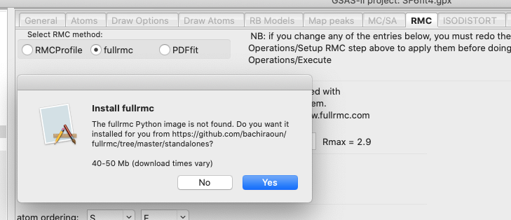
If “Yes” is pressed, a message like the one below in the console window. The file name for the download will vary depending on the type of computer you have and the location where GSAS-II is installed. The download time may vary from many minutes to fractions of a minute. 

 

Starting installation of fullrmc

Downloading from https://github.com/bachiraoun/fullrmc/tree/master/standalones

Creating /Users/toby/G2/trunk/AllBinaries/mac_64_p3.9_n1.19/fullrmc500_3p8p6_macOS-10p16-x86_64-i386-64bit

This may take a while...

...Download completed

 

It is also possible to install this software yourself, from the location where it is made available, https://github.com/bachiraoun/fullrmc/tree/master/standalones. If this is done manually, either install it into the search path described in the GSAS-II help or define the GSAS-II configuration variable fullrmc_exec.

 

It has been seen that the windows .exe file did not run at least one minimal Windows installation without installation of Microsoft-supplied .DLL file(s). Running the file https://aka.ms/vs/17/release/vc_redist.x64.exe from https://docs.microsoft.com/en-us/cpp/windows/latest-supported-vc-redist installs the Microsoft C and C++ (MSVC) runtime libraries and addressed this problem. If any of these binary images do not run for you, we will be unable to help.

 

1. Rietveld Refinement of Sulfur hexafluoride (SF6):

 

This step is optional, but if performed you will follow the steps in RMCProfile Tutorial  I steps 1-6.

 

2. Reverse Monte Carlo Simulation of SF6 with Bond constraints

 

Step 2.1. Import phase

Start GSAS-II. Use the Import/Phase/from GSAS .EXP file menu item to read the phase information for SF₆ into the current GSAS-II project from file SF6_190K.EXP.

 

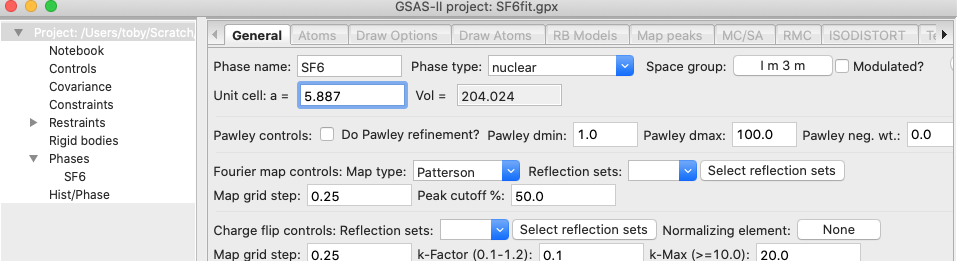
[Alternatively, create a new phase with Space group Im3m (or equivalently Im-3m). While GSAS-II will accept the space group without inclusion of spaces, the correct input would separate the symmetry axes with spaces (I m 3 m). Enter the one lattice parameter, a=5.887. There are two atoms: S atom at 0,0,0 and a F at 0.251,0,0.]

 

Name the phase SF6 and save the project as SF6fit.

 

 

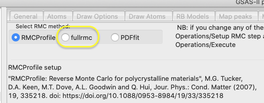
Step 2.2. Setup fullrmc

Select the “SF6” phase tree item, if not already selected; then select the RMC tab. On this window, select fullrmc.

 

 

 

GSAS-II will test to see if a Python interpreter that includes fullrmc is found. If not, you will be offered the chance to install the software, as above. If fullrmc still cannot be accessed, an error message is displayed in the window.

 

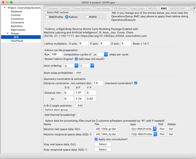
Here we will perform this fit with a quite small superlattice (so that this fit finishes in minutes rather than the hours needed for a better model) and likewise with a relatively small number of steps. We will also use hard constraints on the S-F bond lengths and prevent the SF₆ units from distorting too much, by setting limits on the F-F distances. We will also provide both G(r) and F(Q) input to fit against. To do this provide the following input:

 

·      Use a 5x5x5 supercell by setting the three lattice multipliers to 5

·      Run 100 cycles of 5,000 steps (500,000 steps total). Note that after each cycle, statistics on state of the model are saved for plotting

·      Select to ignore any previous fullrmc runs for this project by selecting the “Restart fullrmc” option (this has no effect for the first fullrmc run for a project).

·      Create distance constraints to place hard limits on the maximum and minimum S-F and F-F distances:

o   In the second column labeled “S-F” set the “min” and “to” values to 1.37 & 1.74

o   In the third column, labeled “F-F” set the “min” and “to” values to 2.0 & 2.42.

·      Load the PDF and structure factor file

o   Use the Neutron G(r) “Select file” button to read the sf6_190_gr.dat file.

o   Since this is a “Keen”-type G(r) as used RMCProfile type, the file type field can be left as the default choice, G(r)-RMCProfile.

o   Use the neutron S(Q)-1 “Select file” button to read the sf6_190_fq.dat file.

o   This is a RMCProfile F(Q) file, which is also the default file type.

Note that these files are slightly different from the versions of the files used in the RMCProfile Tutorial  I. For fullrmc, the first two header lines in the file have been modified to be comments by starting them with a “#” character.

 

When complete, the input should look as below:

 

Step 2.3. Launch fullrmc

Use the Operations => “Setup RMC” menu command. This creates a file containing a script of fullrmc commands named SF6fit-SF6-fullrmc.py, placed in the same directory that was used for the .gpx file. Note that this file is named for both the project (SF6fit) and the phase (SF6).

 

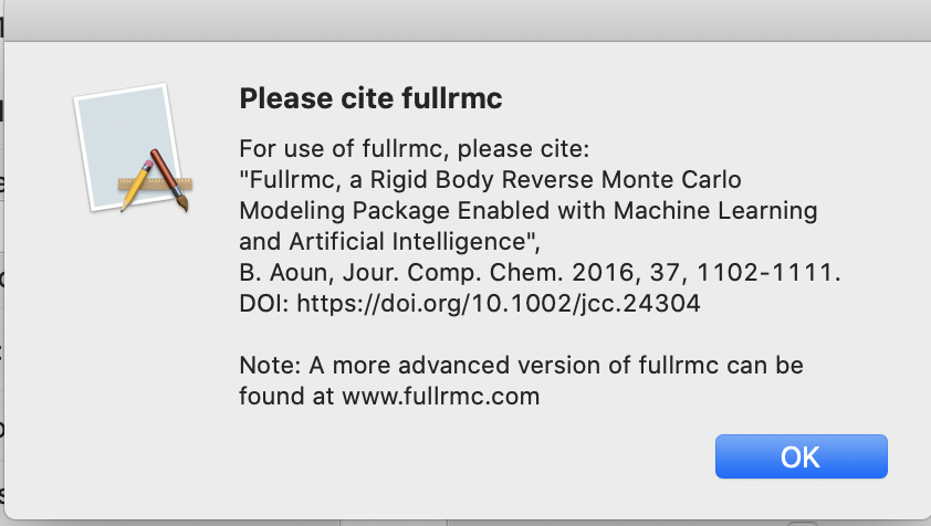
Then use the Operations => Execute menu command to start fullrmc. This creates either a shell script (fullrmc.sh) or a Windows .bat script (fullrmc.bat) to run fullrmc. A reminder on citations is displayed, as below:

 

 

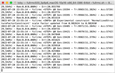
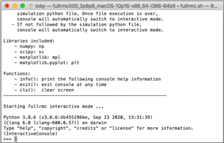
The fullrmc script is then launched in a separate Python process with its own console window. After a brief delay, this will start scrolling status messages:

 

Step 2.4. Plot fullrmc results

Note that in the above input, we selected that fitting would be done with “5K steps/cycle”. This means that every 5000 steps, the fullrmc output is saved so that plots can be generated; it is not necessary to wait for the fullrmc run to complete before plotting results. Use the Operations => Plot menu command to see this output, but notes that these plots are not updated automatically. Repeat the Operations => Plot menu command to update the plots. When this menu command is used, the selection window shown below allows plots to be selected:

 

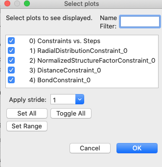
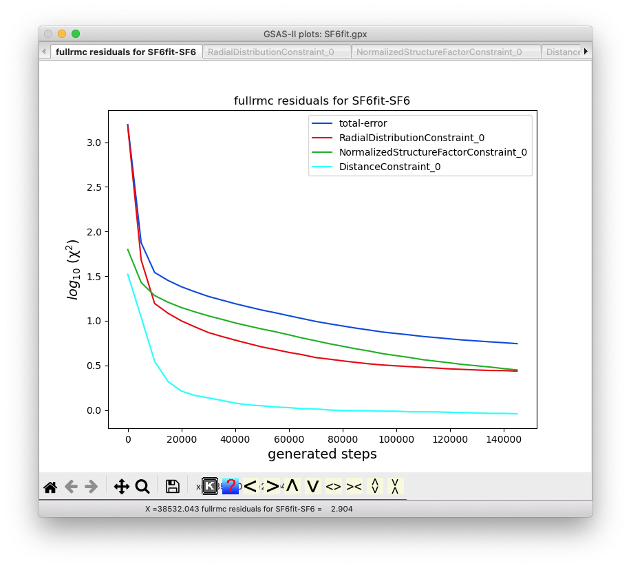
The first listed plot, “Constraints vs. Steps” shows the fullrmc cost functions as the run progresses.

After 10 to perhaps 30 minutes depending on the speed of your computer, the run will complete the 500,000 requested steps. The run of fullrmc is not ended, but rather the terminal window used to run fullrmc remains open and additional fullrmc commands can be typed to create specialized plots or perform other actions within fullrmc.

 

As one example, use of the command

>>> ENGINE.export_snapshot("snapshot.file")

(>>> is a prompt from Python) will create a file with the details of the current model which can be used in fullrmc or transferred to the cloud-based fullrmc system (at fullrmc.com). If the VMD plotting software is installed, the ending atomic configuration can be displayed with command

>>> ENGINE.visualize()

 

To finish fullrmc type:

>>> exit()

 

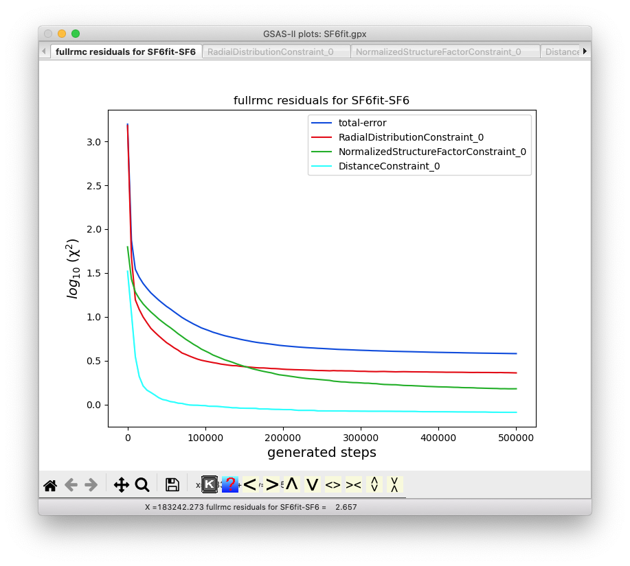
If the Operations => Plot menu command is used after the run of 500,000 steps is complete, the final version of this plot above will appear as below:

 

“Zooming in” on the final section of the plot, as below, shows that the fit quality is still dropping significantly, so even with this relatively small modeling region (5x5x5), 500,000 steps are not enough to optimize the fit.

 

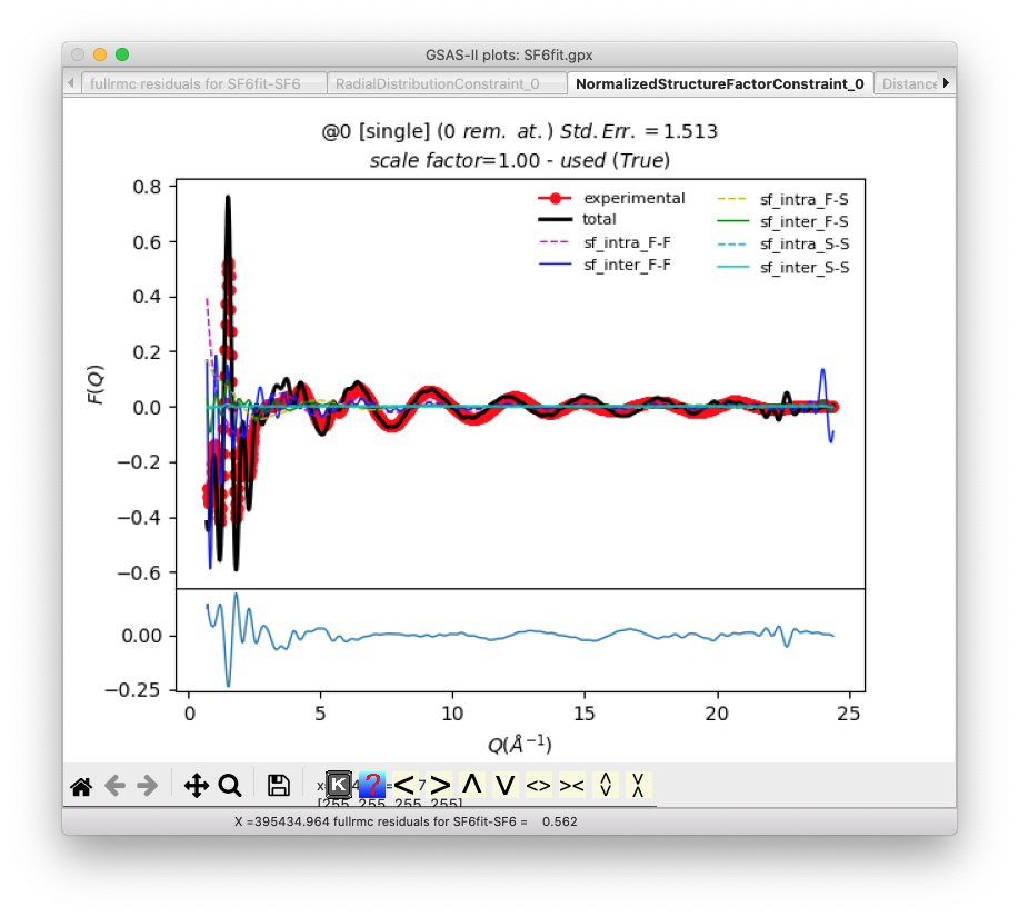
Additional plots show the quality of the fits for G(r) and S(Q):

 

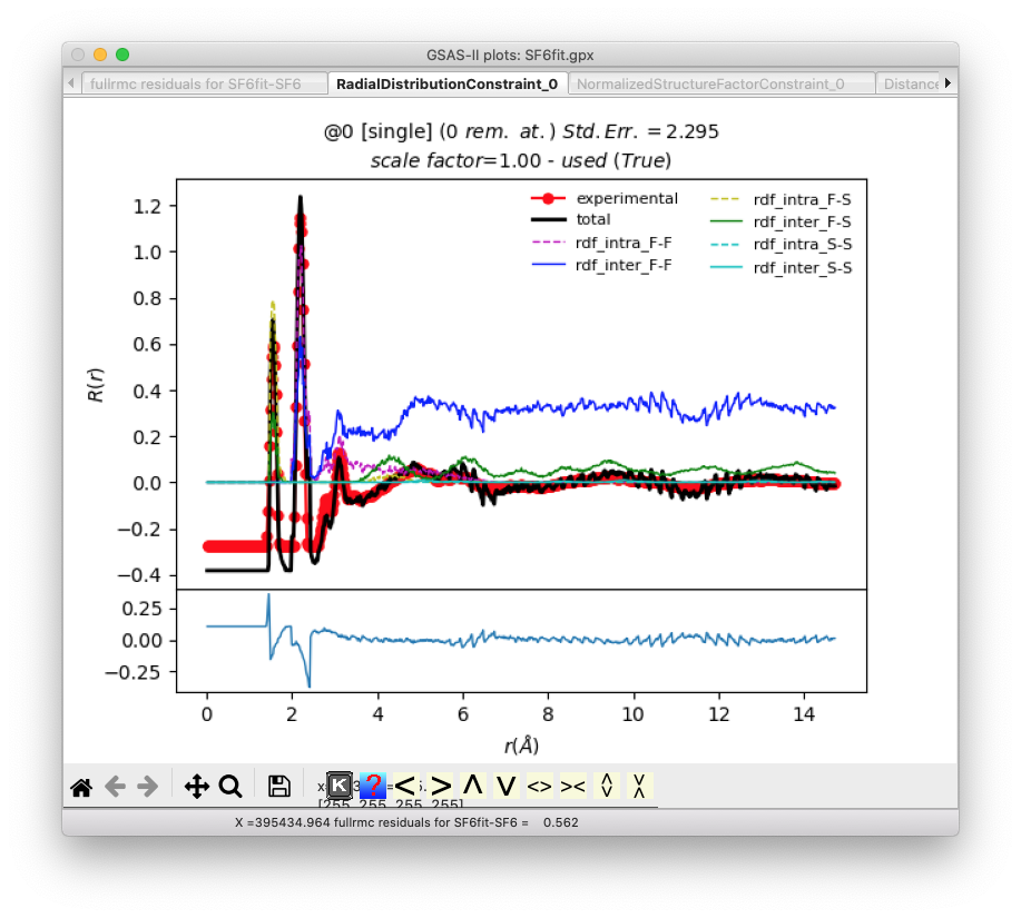
The remaining plots examine the constraints on distances.

 

The run can be continued by unselecting the “Restart fullrmc Engine” and then using Operations => “Setup RMC” and Execute menu commands, but note that with this relatively small modeling space, results will be limited in quality.

 

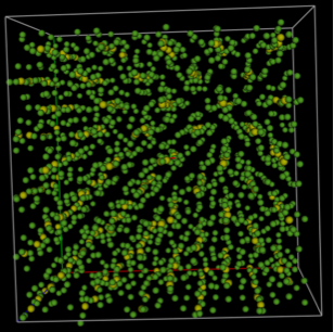
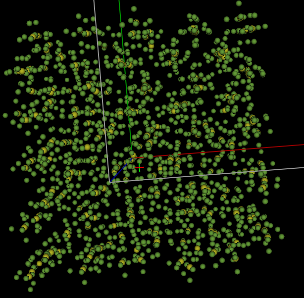
Step 2.5: Transfer fit results inside GSAS-II

The final atom positions generated in fullrmc can be imported back into GSAS-II in one of two ways for viewing or other possible post-analysis. The Operations => “Load Supercell” menu command will input the atoms in the “big box” used for the model as a new phase. Here this will result in a structure with 1750 atoms in a unit cell with 29.4 Å sides. One the fit results are loaded, a new phase named SF6_fullrmc will be created. Click on this phase to view it and then click on the “Draw Atoms” tab to transfer the loaded atoms into the “draw array” then click on “Draw Options” to update the structure plot. The figure below shows the structure after using the sliders to move the “Camera Distance” to ~110 Å, the “Z-clipping” to >35 Å and the “van der Waals scale” to about 0.2.

 

 

 

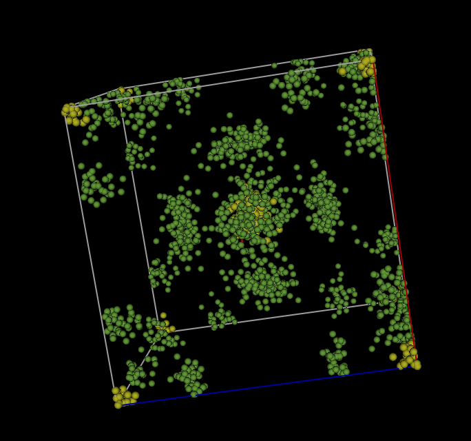
In contrast, the Operations => “Superimpose into cell” menu command places 1750 the atoms from the supercell into the original 5.9 Å crystallographic cell. This menu command must be done from the original “SF6” phase, not the “full cell” phase that was created in the previous step (this is because GSAS-II will look for fullrmc output that is named for both the .gpx file and the phase used to create it.) Since the previous step created phase named SF6_fullrmc, this new phase will be named SF6_fullrmc_1 so that phase names are unique. After clicking on “Draw Atoms” and then “Draw Options,” the “superimposed” cell appears as displayed below, again after the “van der Waals scale” is lowered to about 0.05.

 

 

Step 2.6: Continue the fit (Optional)

Should one wish to see further improvement, the fit can be continued by unselecting the “Restart fullrmc Engine” and then using the Operations => “Setup RMC” and Execute menu commands to continue from where the previous run ended. Note that with this relatively small modeling size, results will be limited in quality.

 

3. Preparation for Rigid Body fitting with fullrmc

 

3.1 Introduction

 

The previous fit in fullrmc, as well as the similar tutorial for RMCProfile, create energetically implausible structures for SF₆ molecules. The reason the previous model is unrealistic is that the packing forces that cause the molecules to shift from the crystallographic high symmetry positions and orientations are too small to cause any significant distortion of the SF₆ molecule from its idealized octahedral geometry. Vibrational modes do allow for instantaneous distortions, by bending the F-S-F angles and stretching/compressing the S-F bonds, these displacements are typically small.

 

The unrealistic model found in RMCProfile as well as here in Step 2, results from the fitting process using atomic shifts to treat two different phenomena, static and vibrational disorder. Even at 0 K, atoms are in constant motion and this gives rise to broadening of PDF peaks. Note that here it is this instantaneous vibrational distortion that broadens the first two peaks, corresponding to the S-F bond and the F-F next-nearest distance, not static disorder. The static displacements of the molecules from their idealized positions could be where the S atoms move from the ideal locations at (0,0,0) and (½,½,½) and/or where the molecule rotates so that the SF bonds are no longer oriented along the unit cell axes.

 

One of the advantages of fullrmc is that it is a framework where nearly any model can be evolved using virtually any protocol that one can devise, but it should also be understood that many features of fullrmc are not available within the GSAS-II GUI. To access the full power of fullrmc one must edit fullrmc scripts manually or use the fullrmc.com interface. Note however, that if GSAS-II does not provide access to desired fullrmc features, the scripts created by GSAS-II may still be of value as a starting point for customized use.

 

In the second part of this tutorial we will use the fullrmc software to pack idealized octahedral SF₆ molecules as rigid units into a supercell but with displacements and/or rotations of these molecules, but we will not allow these units to distort.

 

3.2 Prepare a phase with a single SF₆ Molecule

First, we need to create a single discrete SF₆ molecular unit so that we can designate this as a rigid unit. This requires lowering symmetry. Then we can use this discrete molecule as a building block for our supercell.

 

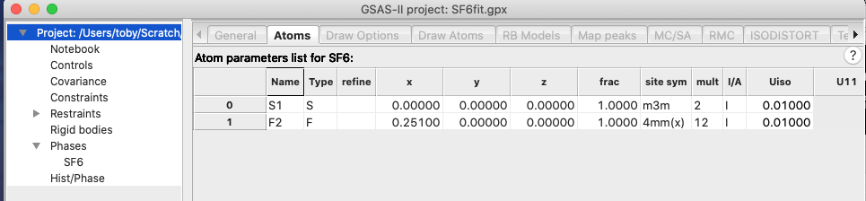
Start by opening the SF6fit.gpx file created in the previous step (or repeat the instructions in Step 2.1 to create the asymmetric unit again.) In the Atoms tab of the SF6 Phase tree entry, note that the asymmetric unit has two atoms, as shown below:

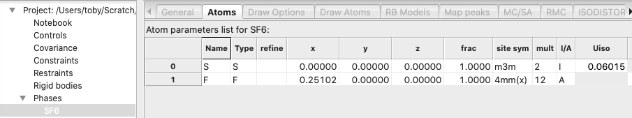
The space group here, Im-3m, has 24 general symmetry operations; these are doubled by a center of symmetry generator and doubled again by the body centering generator, yielding a total of 96 symmetry operations. Both the F and S atoms are on special positions, so that the unit cell contains 2 S atoms and 12 F atoms, as noted by the site multiplicities shown above. If we reduce the symmetry to P 1, we will obtain an asymmetric unit with two SF₆ molecular units. This would work for our purposes, but if we retain the body center and no other symmetry, then we can create an asymmetric unit with a single SF₆ molecular unit. This corresponds to the non-standard – but completely valid – space group of I1, which GSAS-II will accept as input, since space group names are used to generate symmetry by group theory, not from look-up tables (which are not likely to have desired non-standard settings). Creating an asymmetric unit with the single SF₆ molecule we wish is done in two steps:

 

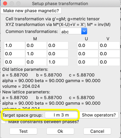
1)   First with the General tab for the SF6 Phase, use the Compute->Transform menu item. We do not need to transform the unit cell, so the M, U & V matrices/vectors are left as the defaults and only target space group must be changed. Click on the target space group button in this window:

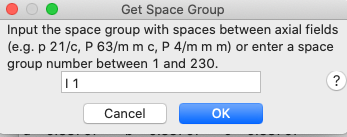
This will open a window for space group input (as below). Enter “I 1” (“i 1” is also fine but note that at least one space between the “I” and the digit “1” is needed so that GSAS-II can interpret the space group properly.)

GSAS-II performs the group theory to derive the generators and operators for this space group and displays them:

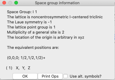
As expected, there is a centering operation, but no other symmetry present.

 

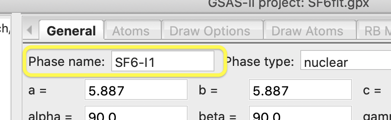
Next, press OK to perform the transformation. A new phase named “SF6 abc” is created (abc here indicates that the a, b & c axes are retained in their original order). To help remind me which phase has lowered symmetry, I renamed this to SF6-I1 with the Phase name entry on the General tab, but this action is optional.

 

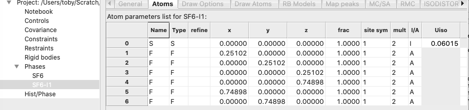
Note that now that the asymmetric unit contains 1 S atom and 6 F atoms, as desired:

 

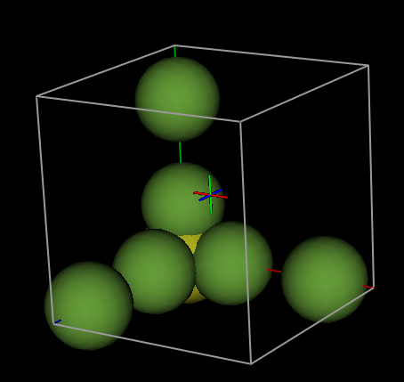
but, selecting the Draw Atoms tab shows us that the asymmetric unit does not yet contain a discrete SF₆ unit:

 

2)   Creating a discrete molecule requires translation of the three “disconnected” F atoms to positions closer to the origin. With the Atoms tab selected, this can be done either the “Assemble molecule” item or the “Collect atoms” item in the “Edit Atoms” menu. The “Collect atoms” option is simpler here. By selecting the Atoms tab and then menu item “Edit Atoms”->“Collect atoms” we can indicate the atoms to be moved to symmetry equivalent positions. Atoms can be selected in the Atoms table, but if no atoms have been selected, this window is shown:

 

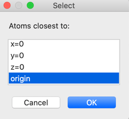
Press the “Set All” button to operate on all atoms and press “OK” (One could also translate only the last three F atoms). In the next window, select that we want to place atoms closest to the unit cell origin. This command will generate all the  symmetry-related positions for each atom, as well as considering unit cell translations and will select from the generated locations the position closest to (0,0,0).

 

and press OK again. The plot now shows what we want, a single discrete molecule:

 

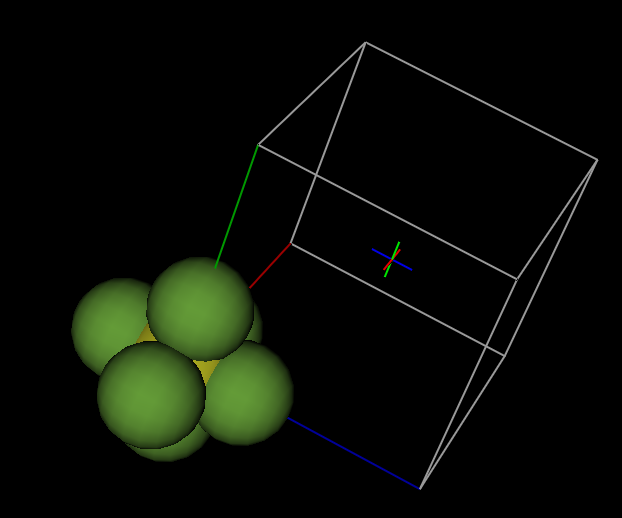
Suggestion: Use File -> “Save Project as…” to save this project under a new name. Here, I used “SF6_I1”.

 

4. Perform a Rigid-Body PDF Fit for SF₆

 

Step 4.1. Setup fullrmc

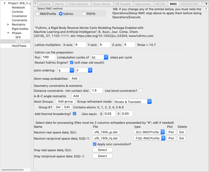
·      Select the new phase, SF6_I1, and change the supercell parameters to 5x5x5 as before and likewise select 100 sets of 5K cycles. Also, as was done in step 2.2, we load the Neutron G(r) PDF, file sf6_190_gr.dat file and the neutron S(Q)-1 file sf6_190_fq.dat.

 

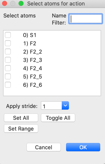
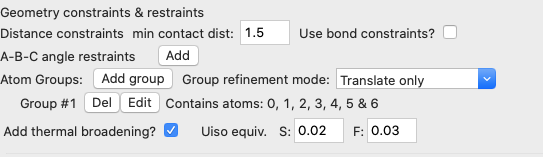
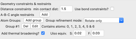
·      However, instead of setting bond distances as bonding constraints, in this simulation we want to define the SF₆ unit as a group of atoms that should be moved as a rigid unit. Note that fullrmc does allow both bond constraints and rigid bodies to be used at the same time, but for this fit this is not needed. Rigid bodies are defined by grouping together the atoms within the body. Do this by pressing the “Define atom group” button. When this is done an atom selection window is opened, as shown below:

 

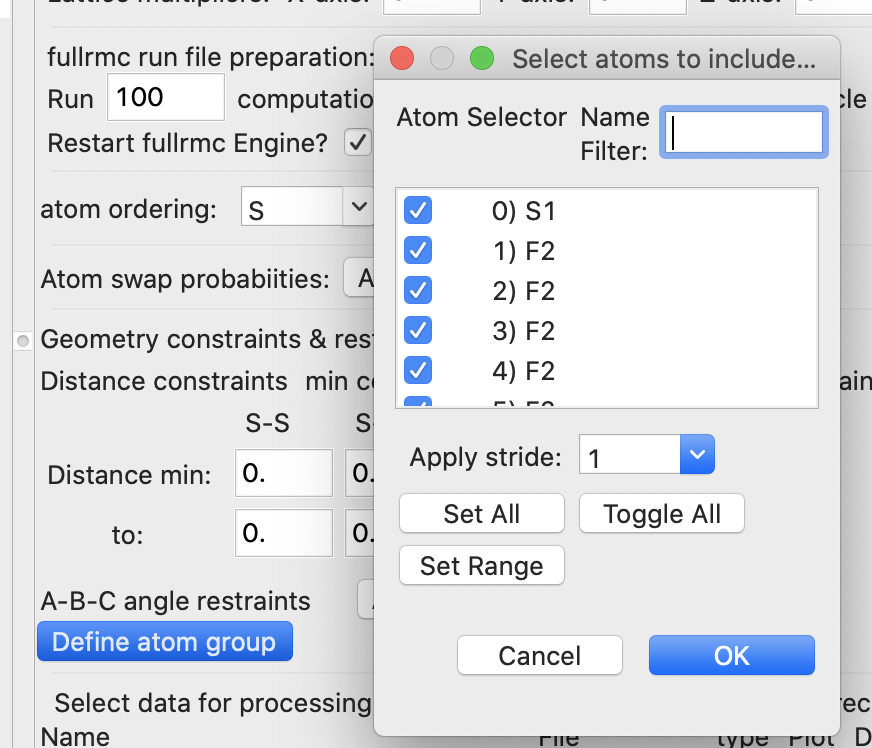
In this window we select all seven atoms will be in the group. Note that now a group is now listed with seven atoms on the fullrmc page (shown below). Also note that the default “Group refinement mode” will both rotate and translate the group.

 

·      We previously used bond-constraints to limit the distortion of the SF₆ molecules, but since they are now rigid units, these constraints are no longer needed. Thus, we can uncheck the “Use bond constraints” box to remove them. Note that leaving the default values of zeros for all distances also causes bond-constraints to be ignored, but the prior choice also simplifies the input screen.

·      We also need to set the vibrational amplitudes for the S and F atoms, by checking the “Add thermal broadening” box. Values to use here are not obvious and might need to be tweaked later, but one would expect more motion from the lighter F atom than the heavier S atom. I used as input values on the order of what I might expect for U_iso for S and F, 0.02 Ų and 0.03 Ų, respectively. The broadening for S-F distances will be the average between the two values.

 

 

 

Step 4.2. Perform fit

As was done in Step 2.3, we launch the fullrmc fit by using the Operations => “Setup RMC” menu command to create a script of fullrmc commands named SF6fit-SF6-I1-fullrmc.py.

 

Then use the Operations => Execute menu command to start fullrmc.

 

Step 4.3. Analysis of results

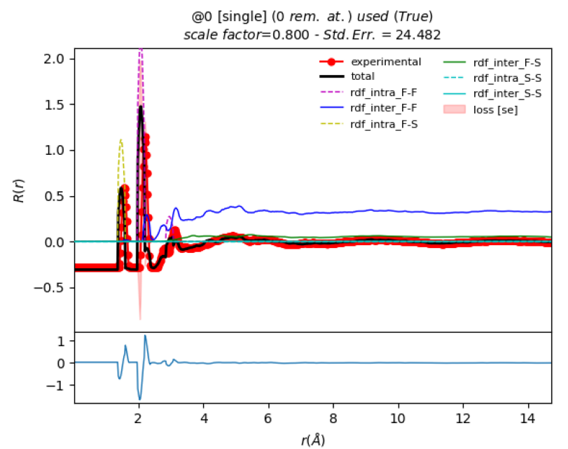
As before, the results can be viewed using the Operations => Plot as well as the Operations => “Load Supercell” menu commands. The PDF and F(Q) are not as well fit as before, but this is expected as the number of degrees of freedom has been reduced by a factor of >3. (Previously there were 3*1750 degrees of freedom, but here only 6*250 are used, because free atoms have three coordinates but rigid groups have three coordinates and three orientation parameters). The fit to G(r) is also showing that the crystallographic fit slightly underestimates the actual bond lengths, as noted by the slight misalignment of the first and second peak, where the first PDF peak is at 1.56 Å but the simulation places it at 1.47 Å.

To obtain plots from fullrmc that can be zoomed, use these commands inside the fullrmc console window:

 

>>> mpl.use('TkAgg')

>>> for c in ENGINE.constraints: p = c.plot(show=True)

...

 

This shortening is expected, as when thermal ellipsoids are used to fit a hollow bowl-shaped distribution of atomic positions, the ellipsoid center is placed inside the “bowl”. This peak displacement could be corrected by repeating this process by editing the F atom x position [from 0.251 to 0.266 (= 0.251 * 1.56/1.47)] in the Im3m setting and then by repeating the commands in steps 3 and 4 above. We will skip this here to save time.

 

Note from the plots the F(Q) Std. Err value is 1.66 and the R(r) Std. Err value is 24.48 (as seen in the plot above).

 

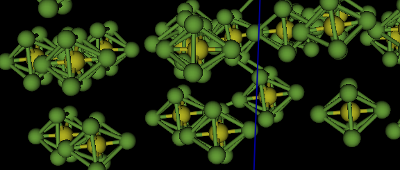
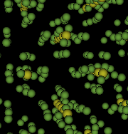
If we load the supercell using the Operations => “Load Supercell” menu command, it shows the expected disorder in the SF₆ molecule positions seemingly as before:

 

 

But, now the SF₆ molecules are no longer distorted. This becomes clear by expanding the scale to look at individual molecules. Optionally, changing the Draw Atoms representation from “vdW balls” to “balls and sticks” (double-click on the “Style” column label) also helps make this clear.

 

 

5. Perform a Constrained PDF Fit for SF6 with Translations only

 

We can compare a model where the molecule center is allowed to move, but unlike before, the molecular axes will not be allowed to move from their alignment with the a, b & c axes by changing the “Group refinement mode” from “Rotate & Translate” to “Translate only”, as shown below:

 

So that we do not overwrite the previous fit, save the project with a new name. Here I use “SF6fitT.gpx”. After running the simulation using the Operations => “Setup RMC” and then the Operations => Execute menu commands to start fullrmc and use of Operations => Plot after completion of the fullrmc run, the results show the F(Q) Std. Err value is 1.73 and the R(r) Std. Err value is 24.15, not very different from the previous result, despite cutting the degrees of freedom by half.

 

Viewing the atoms, and looking closely at different molecules, it becomes clear that the S-F bonds remain aligned with the cell axes, but the molecules are displaced from alignment in columns.

 

6. Perform a Constrained PDF Fit for SF6 with Rotations only

 

We can compare a model where the molecule center is not allowed to move, but unlike before, the molecular axes will be allowed to move from their alignment with the a, b & c axes by changing the “Group refinement mode” from “Translate only” to “Rotate only”, as shown below:

 

Again, so that we do not overwrite the previous fit, save the project with a new name. Here I use “SF6fitR.gpx”. After running the simulation using the Operations => “Setup RMC” and then the Operations => Execute menu commands to start fullrmc and use of Operations => Plot after completion of the fullrmc run, the results show the F(Q) Std. Err value is 12.06 and the R(r) Std. Err value is 28.06, significantly worse that both of the previous results. Thus, we can conclude that rotation of the molecules is less important for a fit to the experimental data than the translation of the molecules.

 

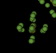
By viewing a column of molecules in this fit, it is seen that the yellow S atoms have remained aligned in columns, but the molecules have been rotated around those positions.

 

7. Conclusions

 

Here we see that the capabilities of fullrmc allows construction and fitting of multiple types of models. While additional work would be needed to create better fits, such as using bigger supercells and running them for much longer, as well as adjustment of bond distances and perhaps the thermal vibration amplitudes, we have seen that we can reproduce much of the features of the experimental G(r) and S(Q) data with a simple model made of rigid SF₆ units that are allowed to translate from their ideal crystallographic site. In contrast, group rotations are much less important. Since these models are much simpler than the models where the SF₆ molecules are highly distorted, but still largely reproduce the experimental results, the simpler models are preferable.