RMCProfile – I

· Exercise files are found here

Introduction

In this and subsequent tutorials, we will show how to use GSAS-II in conjunction with RMCProfile (“RMCProfile: Reverse Monte Carlo for polycrystalline materials”, M.G. Tucker, D.A. Keen, M.T. Dove, A.L. Goodwin and Q. Hui, (2007) Jour. Phys.: Cond. Matter, 19, 335218. doi: https://doi.org/10.1088/0953-8984/19/33/335218) to fit both powder diffraction data and a pair distribution function (PDF) created from it with a “big box” disordered model.

Before getting started you must obtain the most recent Version 6 of the RMCProfile executable (at this writing this is RMCProfile V6.7.9 although V6.7.6 will also work, but not any earlier version). Obtain this from www.rmcprofile.org by following the prompts from Downloads. This version is available for Windows, Mac OSX and Linux. The download will be a zip file; save it somewhere convenient. Pull from it only the RMCProfile_package/exe/rmcprofile.exe and the two files in RMCProfile_package/exe/cuda_lib (if present) and place them in the GSASII main directory or in a new subdirectory (e.g. GSASII/RMCProfile); no other files are needed although you may wish to also retrieve the contents of the tutorial subdirectory. It contains rmcprofilemanual.pdf and rmcprofile_tutorial.pdf which may be of interest since the GSAS-II/RMCProfile tutorials are based on the latter.

The process for using RMCProfile begins with a normal Rietveld refinement of the average structure. For the kind of disordered materials of interest here, this may give bond lengths that are frequently too short for the atoms involved and sometimes extreme apparent thermal motion for some of the atoms. These effects arise because the average structure places these atoms too close to one another; a more localized view would show coordinated atom displacements or reorientation of groups of atoms to avoid the close contacts. RMCProfile is then used to characterize these local displacements by fitting to the diffraction data and its Fourier transform as a PDF.

The material used in this tutorial is the same as described in the RMCProfile tutorial Exercises 1-3, sulfur hexafluoride (SF₆). The average structure of SF₆ is a molecular crystal at low temperatures with the SF₆ octahedra arranged in a body centered cubic lattice with the S-F bonds aligned with the crystal axes. The structural frustration induced by close F-F contacts forces the octahedra to locally rotate in different directions and this disorder gives rise to considerable diffuse scattering. The data used here was obtained at 190K on the GEM diffractometer at ISIS, Rutherford-Appleton Laboratory, Harwell Campus, UK.

If you have not done so already, start GSAS-II.

Rietveld Refinement of Sulfur hexafluoride (SF₆):

Step 1: Read in the data file

1. Use the Import/Powder Data/from GSAS powder data file menu item to read the data file into the current GSAS-II project. This read option is set to read any of the powder data formats defined for GSAS (angles in centidegrees, TOF in µsec). Other submenu items will read the cif format or the xye format (angles in degrees) used by topas, etc. In those cases, you would change the file type to cif format or the xye format to see them. Because you used the Help/Download tutorial menu entry to open this page and downloaded the exercise files (recommended), then the RMCProfile-I/data/... entry will bring you to the location where the files have been downloaded. (It is also possible to download them manually from https://subversion.xray.aps.anl.gov/pyGSAS/Tutorials/RMCProfile-I/data/. In this case you will need to navigate to the download location manually.)

For this tutorial you should see the data file in the file browser, but if extensions on data files are not the expected ones, you may need to change the file type to All files (*.*) to find the desired file.

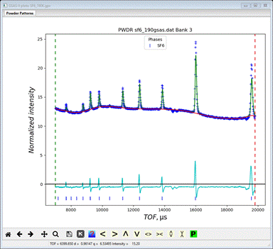
2. Select the sf6_190gsas.dat data file in the first dialog and press Open. There will be a Dialog box asking Is this the file you want? Press Yes button to proceed. The data file contain 3 banks of data

Select only the third one (BANK 3) and press OK. Next will be a file selection dialog for the instrument parameter file; only one is shown. Select it; the pattern will be read in and displayed

There is high background and considerable diffuse scattering at low TOF (high Q) arising from the molecular SF₆ disorder.

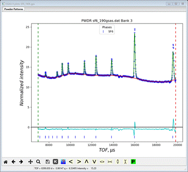
Step 2. Set limits

Because the Rietveld refinement will not make use of the diffuse scattering we want to set the lower limit to just below the first visible Bragg peak; go the Limits entry in the GSAS-II data tree.

Change the 1^st entry to 7000; the plot will change by moving the green dashed line. The upper limit is fine.

Step 3. Import SF₆ phase

The average structure of SF₆ is very simple. Space group Im3m (or Im-3m; same thing), a=5.887 with S at 0,0,0 and F at 0.251,0,0. However, we will save time by importing it from an old gsas experiment file. Use the Import/Phase/from GSAS .EXP file menu item to read the phase information for SF₆ into the current GSAS-II project. Other submenu items will read phase information in other formats. Because you used the Help/Download tutorial menu entry to open this page and downloaded the exercise files (recommended), then the RMCProfile-I/data/... entry will bring you to the location where the files have been downloaded. (It is also possible to download them manually from https://subversion.xray.aps.anl.gov/pyGSAS/Tutorials/RMCProfile-I/data/. In this case you will need to navigate to the download location manually.) Select the SF6_190K.EXP file (only one there) There will be a Dialog box asking Is this the file you want? Press Yes button to proceed. You will get the opportunity to change the phase name next (I left it alone; NB: because of restrictions in RMCProfile it is important that the phase name not have any spaces); press OK to continue. Next is the histogram selection window; this connects the phase to the data so it can be used in subsequent calculations.

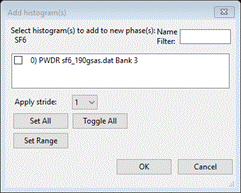
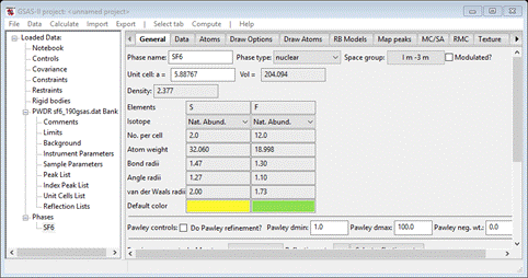
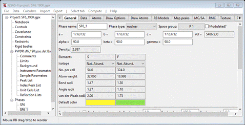
Select the histogram (or press Set All) and press OK. The General tab for the phase is shown next

Step 4. Set the background

Because there is considerable diffuse scattering, the default background will be insufficient for reasonable fitting. Select the Background item from the GSAS-II data tree

Be sure that “chebyschev-1” is used for the background function; RMCProfile only recognizes that form to compute the background for the diffraction pattern. Select 15 for the number of terms.

Step 5. Rietveld refinement

We are now ready for the first Rietveld refinement; select Calculate/Refine from the main GSAS-II menu. Before it starts a file selection dialog will appear; select a file name (no extension). I chose “SF6_190K”; do not use the phase name for this purpose because RMCProfile will use that as the root for the many files it creates. Also, you should create a new directory for this exercise while in this dialog box; it will be rapidly filled up with RMCProfile files which can lead to considerable confusion if mixed in with other files. For Windows after navigating to a suitable location, a new directory can be made by a right mouse click and selecting “New/Folder” from the popup menu. It will appear with the name “New Folder”; change the name and select it (it will be empty). Other operating systems will have similar methods. Finally press OK to save the GSAS-II project (SF6_190K.gpx) and start the refinement. It will quickly converge to give a quite low Rwp (~2.2%) mostly because of the very high background

It is evident that the lattice parameter needs adjusting. Go to the General tab for the SF6 phase and select Refine unit cell; repeat Calculate/Refine. The Rwp will improve (~0.76%) giving

To finish up add the following parameters:

SF6/Atoms: XU for both atoms (GSAS-II recognizes that the S atom is fixed in position); the F atom should have anisotropic thermal displacements.

SF6/Data: refine microstrain and set size to 10.

PWDR/Instrument Parameters: refine beta-0, beta-1, sig-0, sig-1 and sig-2 (normally not necessary, but the available GEM instrument parameter file isn’t current). In any event, the coefficients difB, beta-q and sig-q must be zero since RMCProfile V6.7.6 Beta Serial does not know how to use them in computing a powder profile.

Do Calculate/Refine from the main menu; the fit will quickly improve a bit more to Rwp ~ 0.56%.

Step 6. Draw structure

Select the Phases/SF6/Draw Atoms tab; the list will be shown and the two unique atoms drawn on the plot.

To improve this do the following:

1) Double click the Style column heading and select ellipsoids; the figure will be redrawn showing the 50% ellipsoid surfaces.

2) Double click the empty upper left box in the Draw Atoms table; both atoms will turn green and the two table rows will be grey.

3) Under the menu Edit Figure select Fill unit cell; the figure will be redrawn showing all atoms in the cell (too many bonds, though).

4) Double click the Type column heading and select the S atom type

5) Under the menu Edit Figure select Fill CN-sphere; the figure will be redrawn with six F atoms about all S atoms (still too many bonds).

6) Finally select Draw Options tab and change Bond search factor to 0.7; the figure will be redrawn to show

which is what one expects for orientational disorder for the SF₆ molecules. Next we will explore this with a RMCProfile simulation. To keep this drawing, you may want to save the GSAS-II project.

Reverse Monte Carlo Simulation of SF₆

RMCProfile is most effective if a large box is used for the modelling; this requires very long running times (10-20 hrs for SF₆) before a meaningful result is obtained. However, for the purposes of this tutorial, we will be using a smaller big box model that converges in a more reasonable time (~10min). The result will clearly fit the data but the model is too small to give enough molecular orientations to be meaningful, however this exercise will show you how to set up RMCProfile from within GSAS-II.

To start select the Phases/SF6/RMC tab; if rmcprofile.exe is within the GSASII directory the data window will show

At the top is a radio button selection for RMCProfile and fullrmc. The latter is an alternative big box modeling program (not working – under development); RMCProfile is selected by default and all below are its setup controls. There are four major sections (metadata, major controls, restraints & constraints and data controls); we will work through each of these in turn. The information you enter here is retained in the GSAS-II project so you can easily try alternative setups without having to enter everything over again.

Step 1. Set metadata items

The entries here are for your convenience; there is no explicit use made of any of these, but they will appear in some of the output files from RMCProfile and of course will show here on subsequent views of this window. Fill out as many of them as you see fit. I entered some things for each as the defaults are somewhat nonsensical.

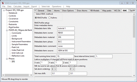
Step 2. Set general controls

The running time is defaulted to 10 minutes with a Save interval of 1 minute. At each save time a number of files are written by RMCProfile; these can be viewed by using the Operations/View command (more about this later – don’t bother trying it now, there is nothing to see). For the purposes of this tutorial leave them at their defaults.

The big box model used by RMCProfile is described as multiples of the unit cell axes. In this case we want a 3x3x3 box so enter 3 for each of X-axis, Y-axis and Z-axis.

Next is to set the order of the atom types in the structure; this is used to construct atom-atom distance restraints on the modelling. The order here (S followed by F) is appropriate; if changed the window will repaint updating various entries possibly resetting some entries to defaults. I suggest you decide the order now and then don’t change it later. Set the maximum shift for S to be 0.05 (the value for F is OK). When done the window should look like

Skip the next item (Atom swap probabilities). This is for cases in which atoms can exchange sites.

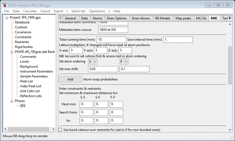
Step 3. Set constraints/restraints

Next is to set the “Hard” minimum atom-atom separation and the allowed search rage for each pair. Enter 4, 1.37 and 2 for the S-S, S-F and F-F Hard min. This rejects any proposed atom move that results in a contact less than that value.

The search range further restricts the allowed moves; this can maintain bonding within the structure. Enter 1.37 & 1.74 for the S-F Search from and to values, and 2.0 & 2.42 for the F-F values. The window should look like

Scroll down to the bottom of the window for the last section.

Step 4. Select data to be fitted

We will be using three different types of SF₆ data for the fitting by RMCProfile. The first is the selection of the powder pattern (“Bragg”) for processing. This is taken from the PWDR entries in the GSAS-II project and accessed from the pulldown; there is only one “PWDR sf6_190gsas.dat Bank 3” that was used earlier in your Rietveld refinement of SF₆. If you had used multiple banks in the Rietveld refinement, all would be shown in the pulldown, but only one can be selected. Set the weight to 0.1 (NB: smaller numbers means a heavier weight).

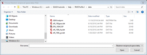
Next press the Select button for the “Neutron real space data; G(R)” line; a FileDialog should appear. Because you used the Help/Download tutorial menu entry to open this page and downloaded the exercise files (recommended), then the RMCProfile-I/data/... entry will bring you to the location where the files have been downloaded. (It is also possible to download them manually from https://subversion.xray.aps.anl.gov/pyGSAS/Tutorials/RMCProfile-I/data/. In this case you will need to navigate to the download location manually.)

The FileDialog should show

Select sf6_190k_gr.dat; it will be copied from this location to your working directory for this tutorial (RMCProfile requires all its files to be local). The window will be redrawn showing the new entry; the weight is fine.

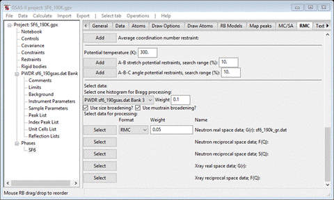
Next press the Select button for “Neutron reciprocal space data: F(Q)”; the FileDialog will show

Select sf6_190k_fq.dat; again it will be copied to your working directory. The window will be redrawn

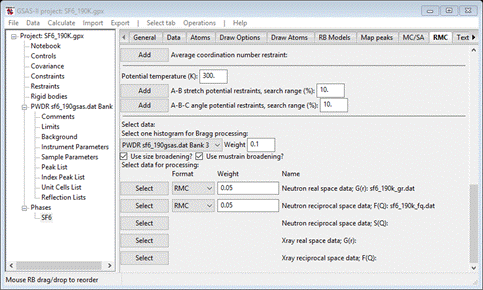
Change the weight to 0.01. Your local directory should have just 3 files

Step 5. Setup RMCProfile files

You are now ready to setup the RMCProfile input files.. Do Operations/Setup RMC from the menu; the console should report that files were written

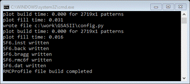
and your local directory should now have 8 files

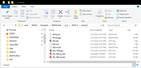
These text files contain data needed by RMCProfile for the fitting of SF6. They are:

SF6.back- the 15 coefficients for the chebyschev-1 function needed to comput the background for the Bragg pattern

SF6.bragg – the powder pattern used in the Rietveld refinement

SF6.dat – the RMCProfile controls file; described in full in the RMCProfile User Manual. It can be edited if need be, but remember it is rewritten each time Operations/Setup RMC is done.

SF6.inst – the instrument parameter coefficients for the neutron TOF peak shape function used by GSAS-II and implemented in RMCProfile for computing the Bragg pattern.

SF6.rmc6f – the big box set of atom positions. It is normally not rewritten when Operations/Setup RMC is done unless the X-axis, Y-axis, or Z-axis lattice multipliers are changed. Most important is that it will contain the set of big box atom positions as updated by RMCProfile according to the Save interval (every 1 min in this case).

You are now ready to run RMCProfile.

Step 6. Run RMCProfile

To run RMCProfile from inside GSAS-II, do Operations/Execute. You will first see a “nag” note asking you to cite the publication describing RMCProfile; press OK.

The program will start in a new console window – processing will initially be pretty fast for this case and then slow down as the modelling proceeds. It reports Time used and Last saved. Once the latter is nonzero you can view intermediate results to see its progress. Note that you can exit GSAS-II and RMCProfile will continue running. After RMCProfile finishes note that the project directory now has ~30 files many of which are just temporary ones created by RMCProfile. We will be looking at just the *.csv files and the SF6.rmcf6 file; the latter contains the last atom configuration acceptable by RMCProfile thus representing a best disordered model.

Step 7. Viewing results from RMCProfile

Do Operations/View; a FileDialog showing only *.csv files will appear

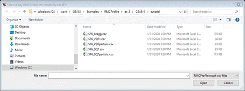
They all should have the same prefix in their name, “SF6” which is the phase name from the GSAS-II project file. Select any one of them – it doesn’t matter. All of them will be read and their contents displayed as individual plots. For example the chi^2 plot shows the progress of the RMCProfile fit

The inset is the upper 3/4ths of the plot magnified; you can see that RMCProfile is still improving the fit slowly even after 10 minutes of running.

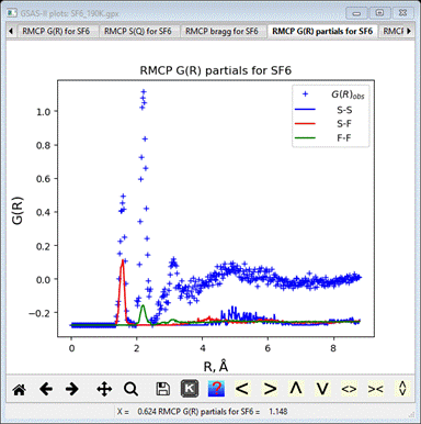
The G(R) partials plot shows the identity of each feature; the first 2 sharp peaks arise from S-F (1.58Å) and F-F (2.20Å) distances within the SF₆ octahedron (cf. 1.457Å and 2.06Å, respectively, for the average structure) while the broader one at 2.8-3.1 are from F-F intermolecular contacts.

Comparing the Bragg plot with the PWDR plot shows that the RMCProfile fit is very similar to the Rietveld fit

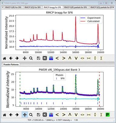
This plot was made by dragging one plot tab to the bottom of the screen to create the second frame.

Step 8. View the big box structural model for SF₆

Next, we can view the resulting big box structure. Do Import/Phase/from RMCProfile .rmc6f file; a FileDialog box with one entry will show the required file, SF6.rmc6f. You will first see a Is this the file you want popup window; select Yes. Next will be an Edit phase name popup. The proposed name is the same as the existing one; GSAS-II will rename this one by adding ‘_1’ to the end. Next will be a popup for Add histograms; respond Cancel because you don’t want this phase to be in any subsequent Rietveld refinement. Looking at the General tab for this phase we see it is 3X in all three axes relative to the original and has no symmetry (space group P 1).

Select the Draw Atoms tab for this phase; a van der Waals ball model will be drawn. You can select the S atoms & fill the CN-sphere for them (does take time – be patient) and then change all the atoms to ball and stick style. The CN-sphere filling works because the RMCProfile structure still has translational symmetry across its 3x3x3 lattice. You should see something like

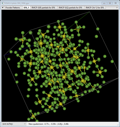
Notice the rotational disorder as well as some positional shifting of the SF₆ molecules. The stray F atoms are bound to SF₆ molecules in neighboring boxes.

NB: this import facility can be used to load any rmc6f file, e.g. from a RMCProfile run done outside of GSAS-II; all the plotting and tools in this and the following steps are available for these big box models.

Step 9. View the disordered average structure

We can compress the big box result back into the original average crystal structure to see how the disordered sites compare with the average ones. Select the General tab for the big box phase (SF6_1) and then do Compute/Transform. A popup dialog will appear

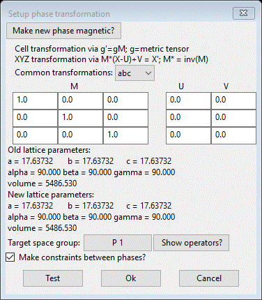
This is the general tool inside GSAS-II for all sorts of structure transformations. Here we will use it to push all the big box atoms back into the average structure unit cell. Recalling that the big box model is 3x3x3 the original unit cell, we simply want to reverse the process. Enter 1/3 into the diagonal elements of the M matrix. The GUI will convert them to the decimal equivalent (0.333…). The target space group should be P 1. You should see

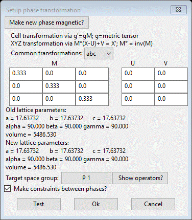
Press Ok to do the transformation. A new phase, “SF6_1 abc” will be formed as triclinic with cell axes that match the original cubic ones. Select Draw Atoms; a van der Waals model will appear.

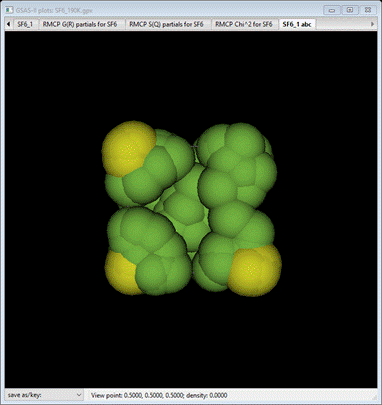
Select the Draw Options tab and reduce the van der Waals scale to about 0.05.

This compares pretty well with the original structure with the ellipsoids drawn at 90% probability.

Step 10. Polyhedral comparison for the big box model

In this step we will examine how the suite of SF₆ molecules deviate from an ideal octahedron. This analysis is currently restricted to structures with P1 space group symmetry; this is what we have from Step 8 above. Select Phases/SF6_1 from the data tree; the General tab will appear.

What we want is at the bottom of this panel; scroll down to the bottom

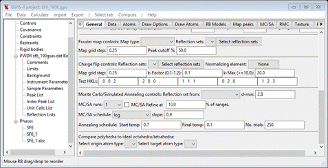
At the very bottom is the control for polyhedral comparison. All that is needed is to select the central atom (“origin atom type”) and the polyhedral vertices (“target atom type”). Select S for the former and F for the latter. Then do Compute/Compare from the menu; a popup for setting Distance Angle Controls will appear

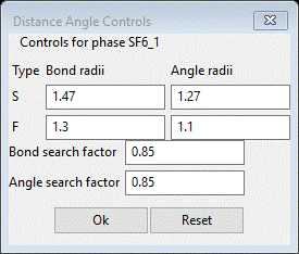
In some cases the bond search factor may need to be adjusted to get the right number of vertices for the polyhedral; in this case 0.85 is fine (NB: in this use the angle ranges are ignored). Press OK; a progress bar will show the atoms being processed. The console may show some atoms being skipped because the number of vertices wasn’t either 4 (tetrahedron) or 6 (octahedron); all are ok here. In this case it quickly finishes; for larger big box models this calculation can take a number of minutes. The General tab reappears already scrolled to the bottom

A new button (Show Plots?) has appeared after the atom selections; press it. A number of new entries will appear on the plot window; we will discuss each in turn. Select the Bond tab

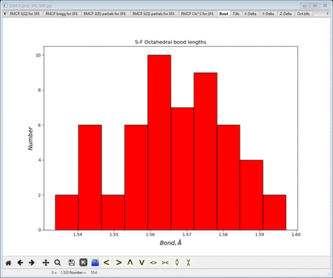
This gives the distribution of S-F bond lengths for all the polyhedral found across the big box model. It is rough because of the small size of the model. The console will have listed the average value with the standard uncertainty in parentheses.

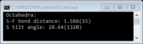
Next select the Tilts tab

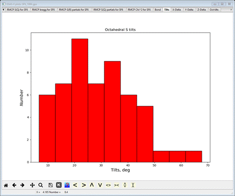
This gives the distribution of axial tilts of the SF₆ molecules from the reference octahedron (aligned along the Cartesian axes). There is a wide distribution with a roughly average tilt of ~30 deg (the average tilt is also shown on the console). Next select X-Delta, Y-Delta and Z-Delta tabs in turn.

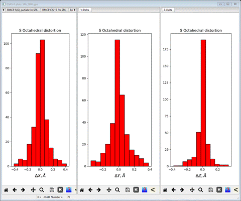
I have made this plot by dragging the respective plot tabs to one of the right (or left) edges to create a 3 pane plot. These show the displacement of the F atoms from the ideal octahedral vertices along each Cartesian axis. Here they are arranged about the zeros fairly tightly. If there were structural distortions to the octahedra (e.g. Jahn-Teller distortions) these could show in these plots. Finally select the Oct tilts tab; a 3D plot will be shown

The sticks marks show the directions of the unit vectors about which the SF₆ molecules are tilted with respect to the reference octahedron and the colors indicate the angle of rotation according to the color bar on the right. In this case they are quite random; they cover all directions and rotations. Note that the algorithm selects the shortest F atom to octahedral vertex for the tilt calculation. That could be any one of the six possible along +/- xyz axes.

This completes this RMCProfile tutorial; you should save the project.

Final note

A production run with enough atoms to give decent statistics would be for a box that is 10x10x10 the original unit cell and would require a 10-20 hour run time. It would contain ~14000 atoms instead of 377 as used here.