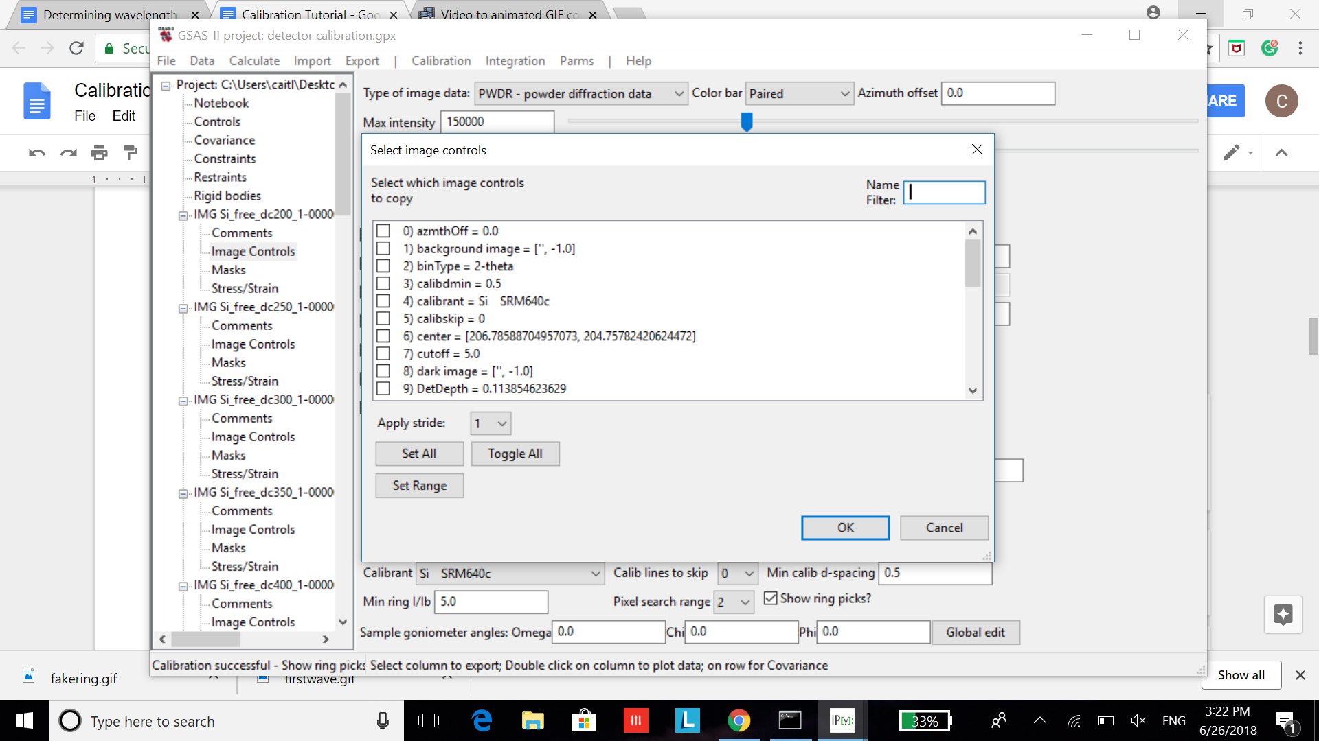
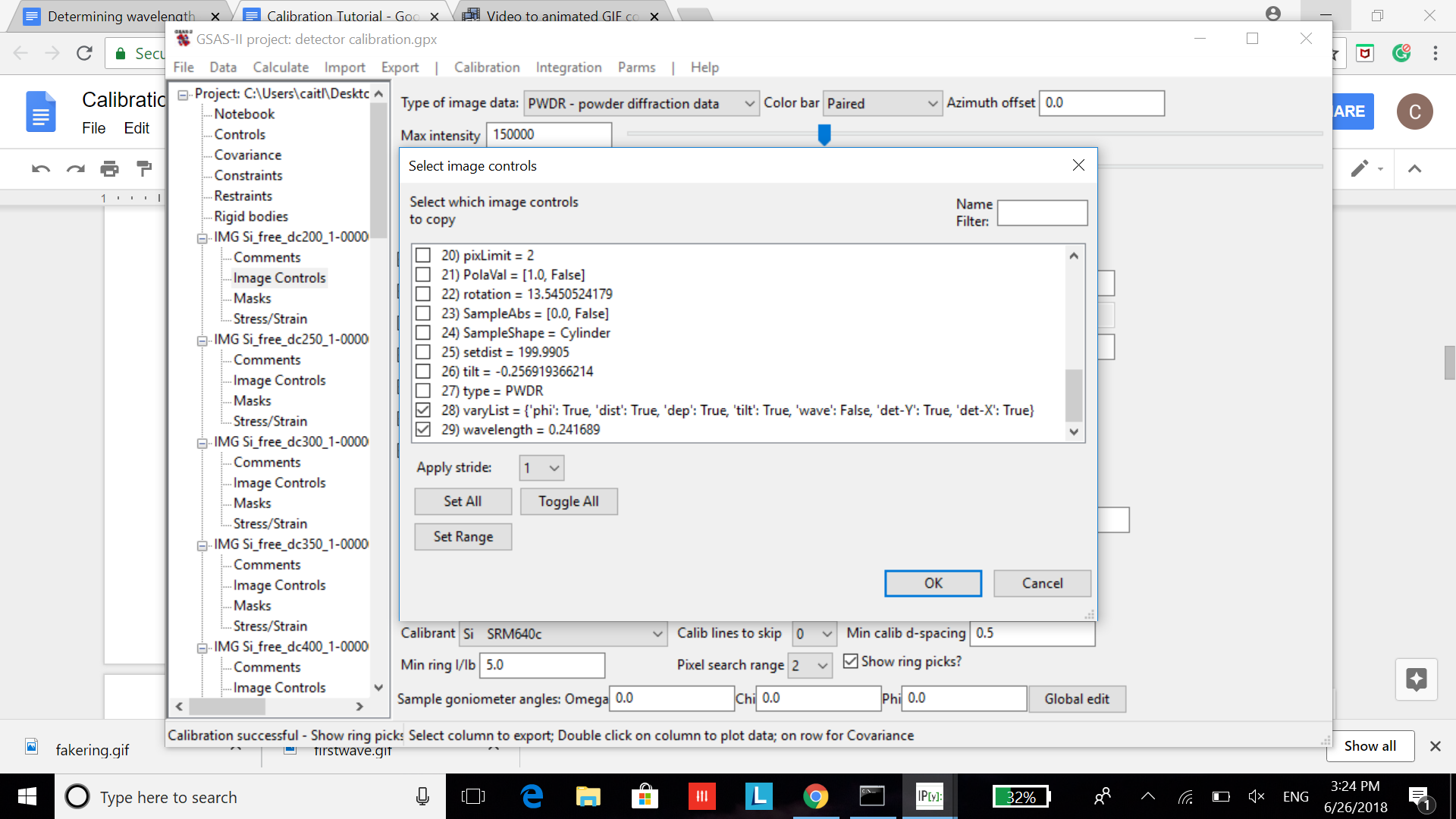
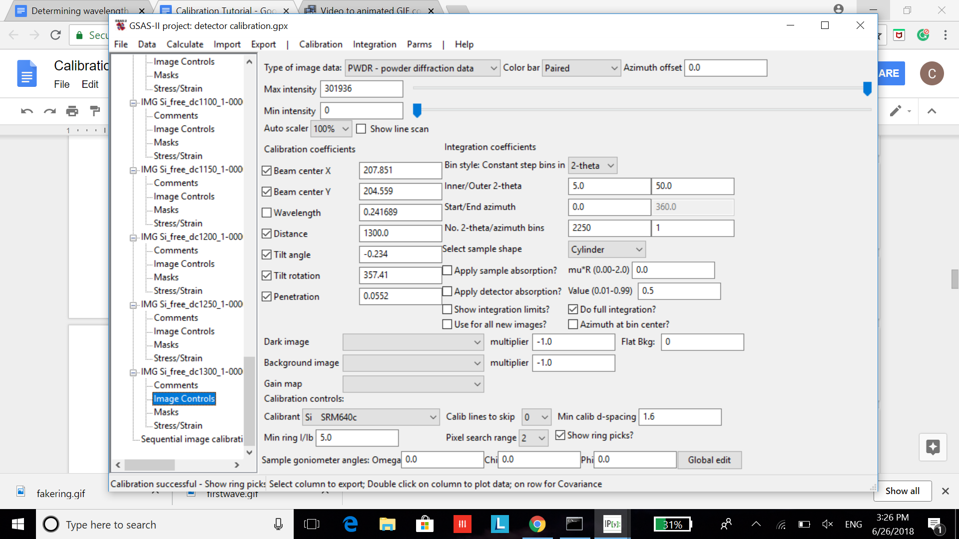
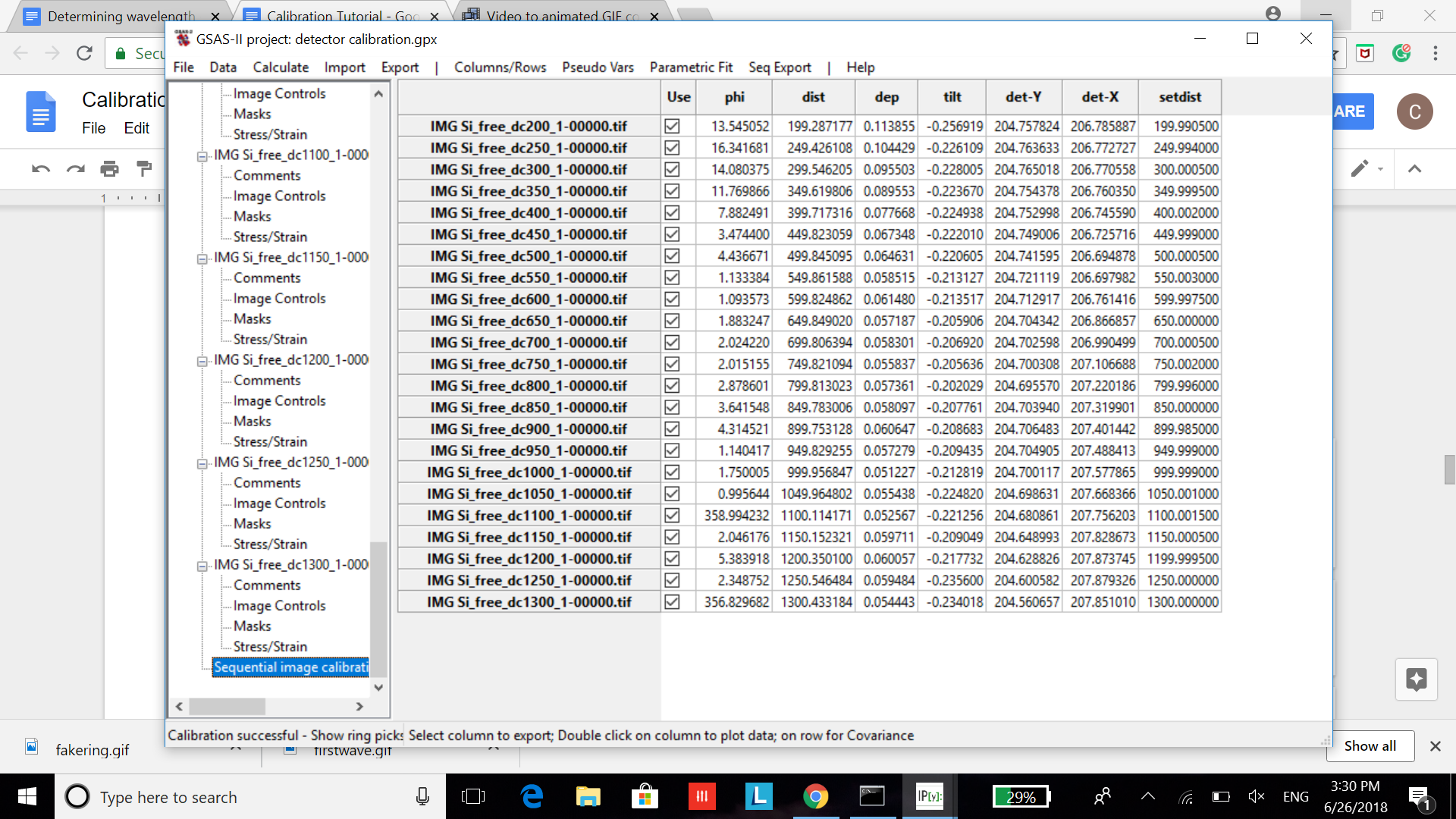
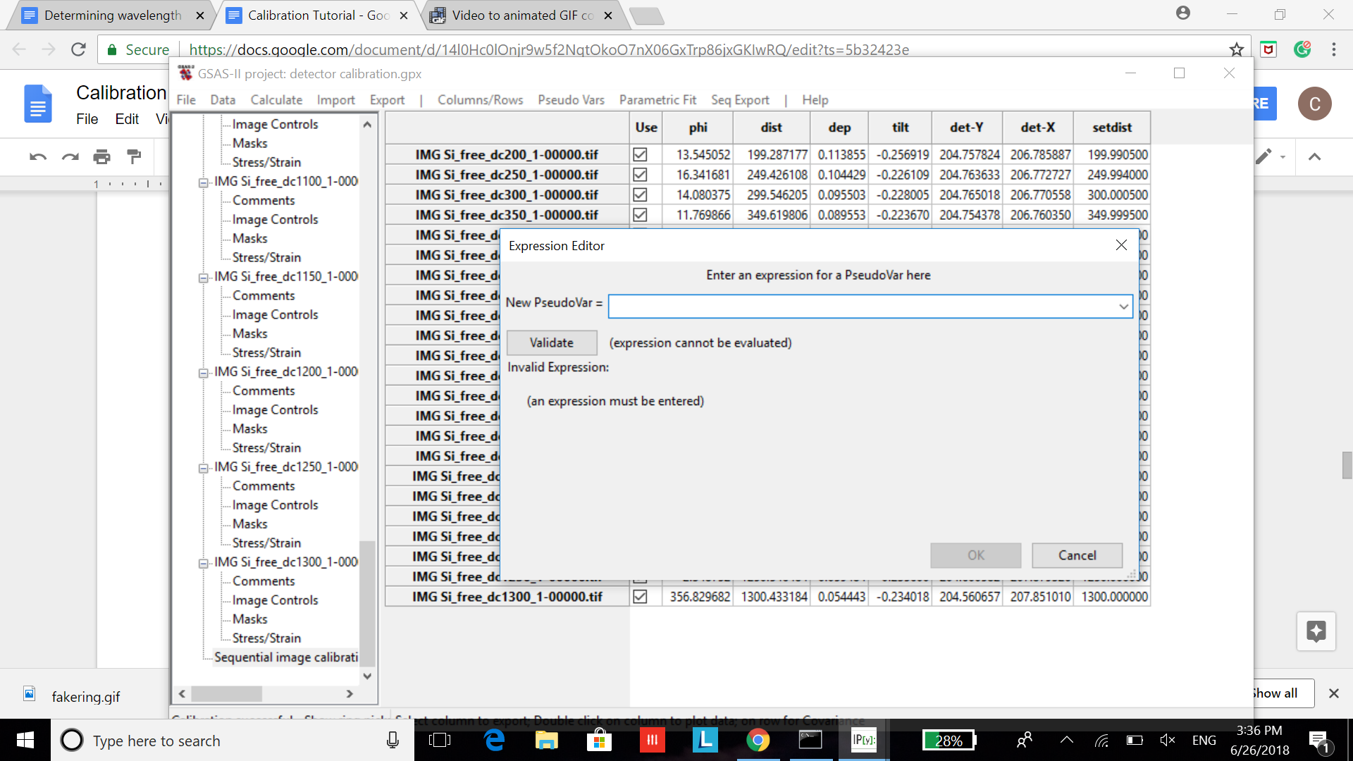
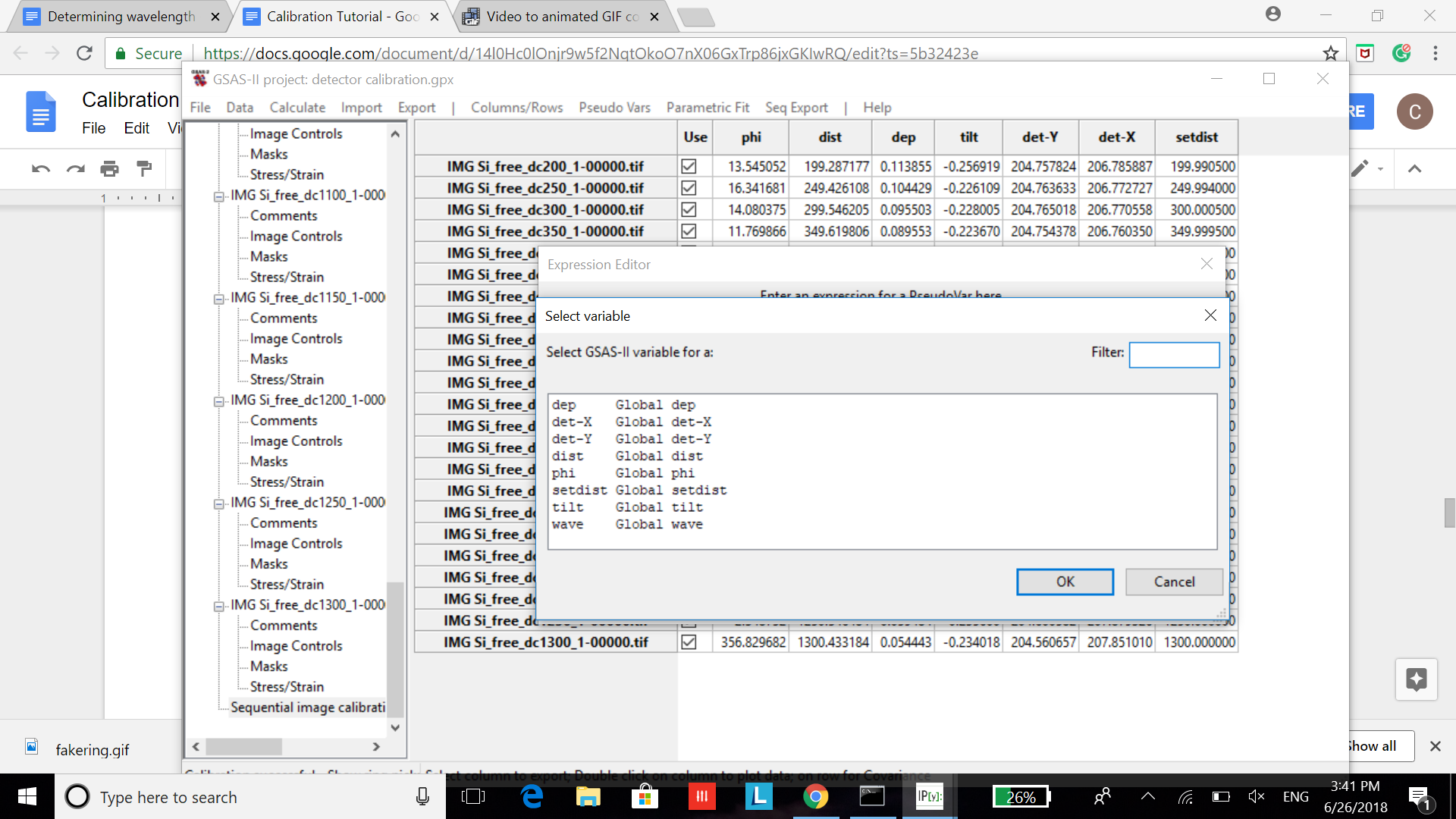
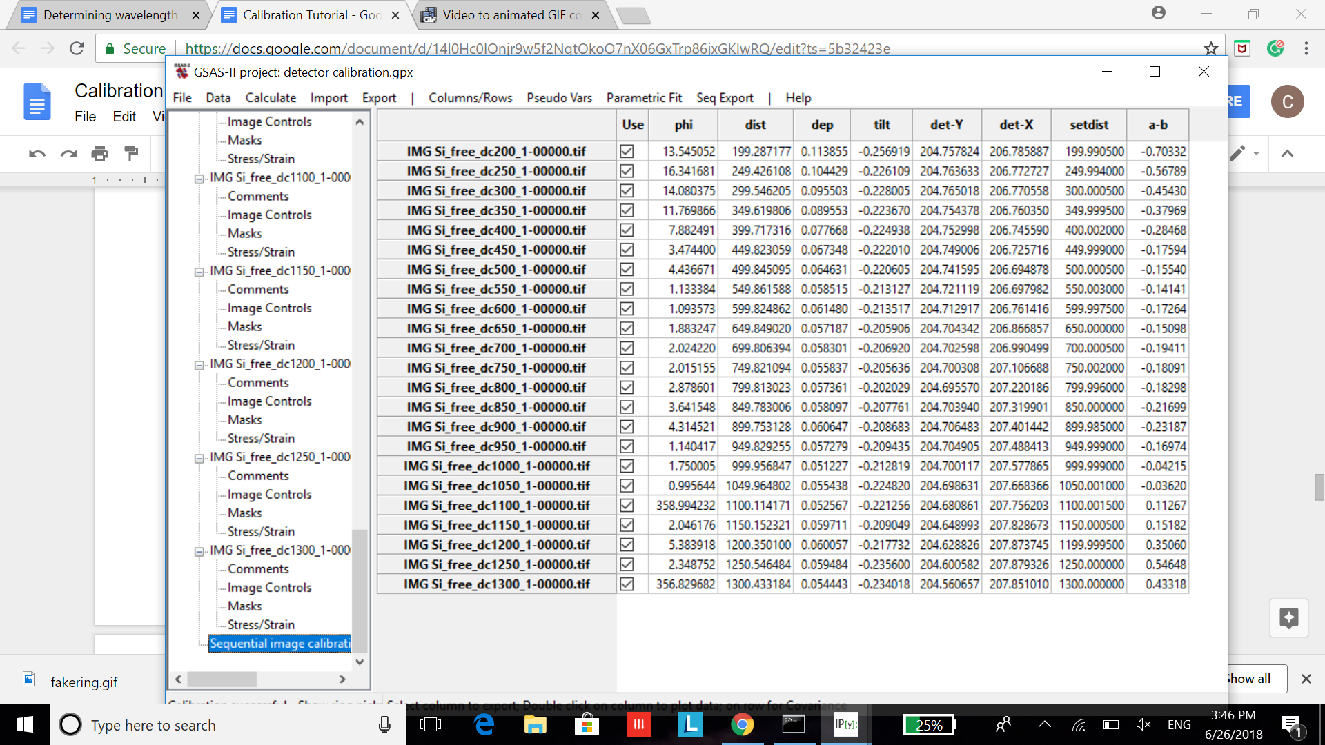
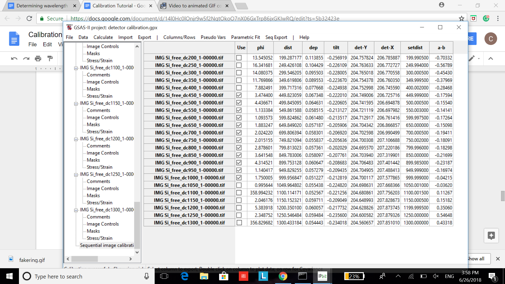
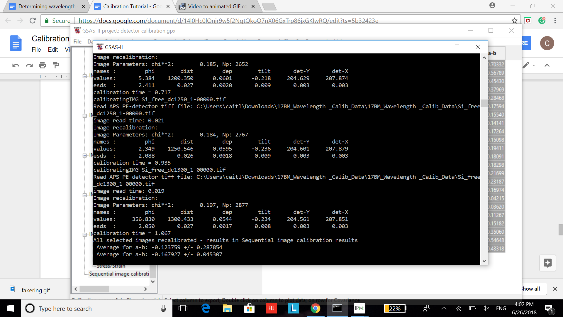
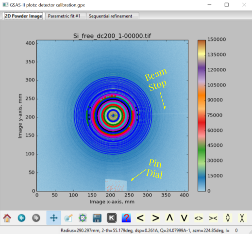
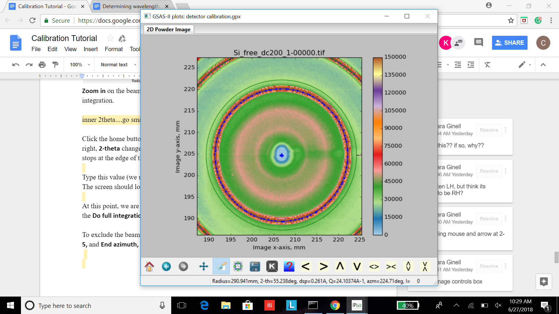
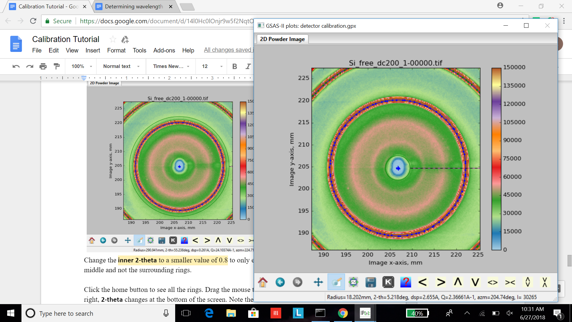
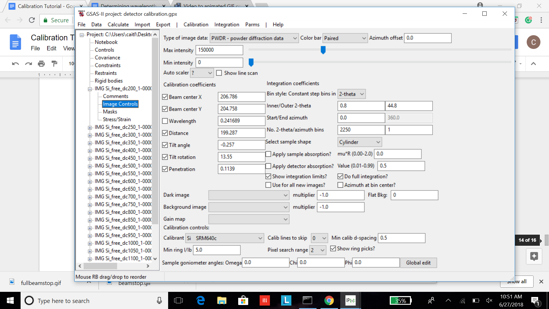
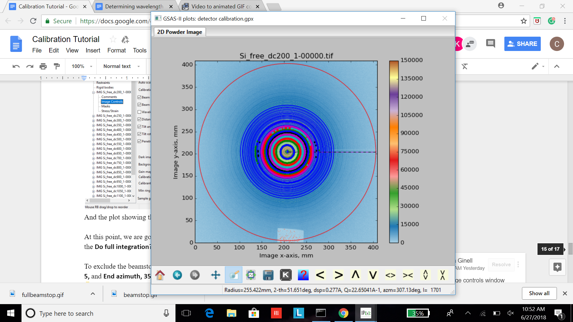
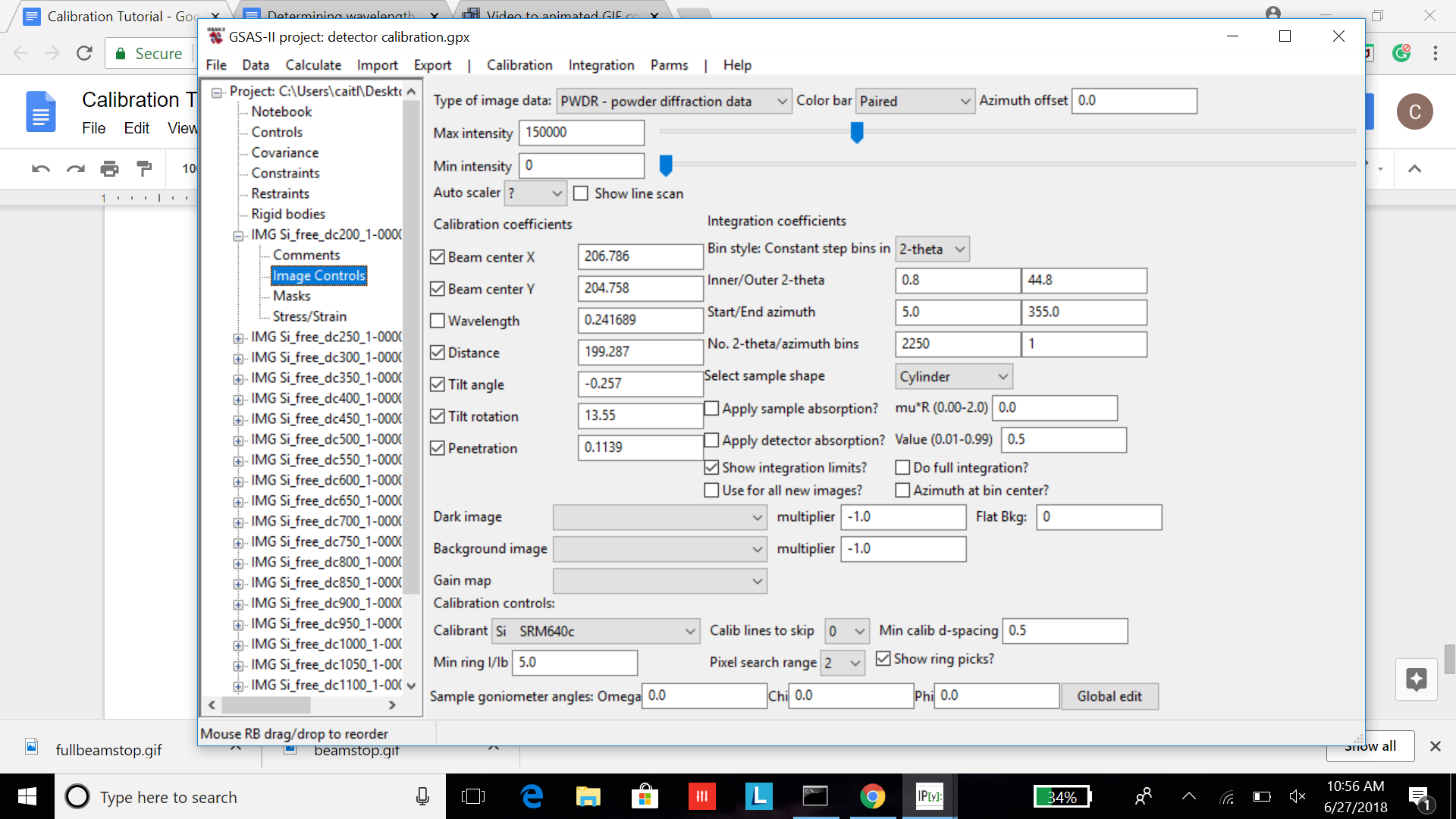
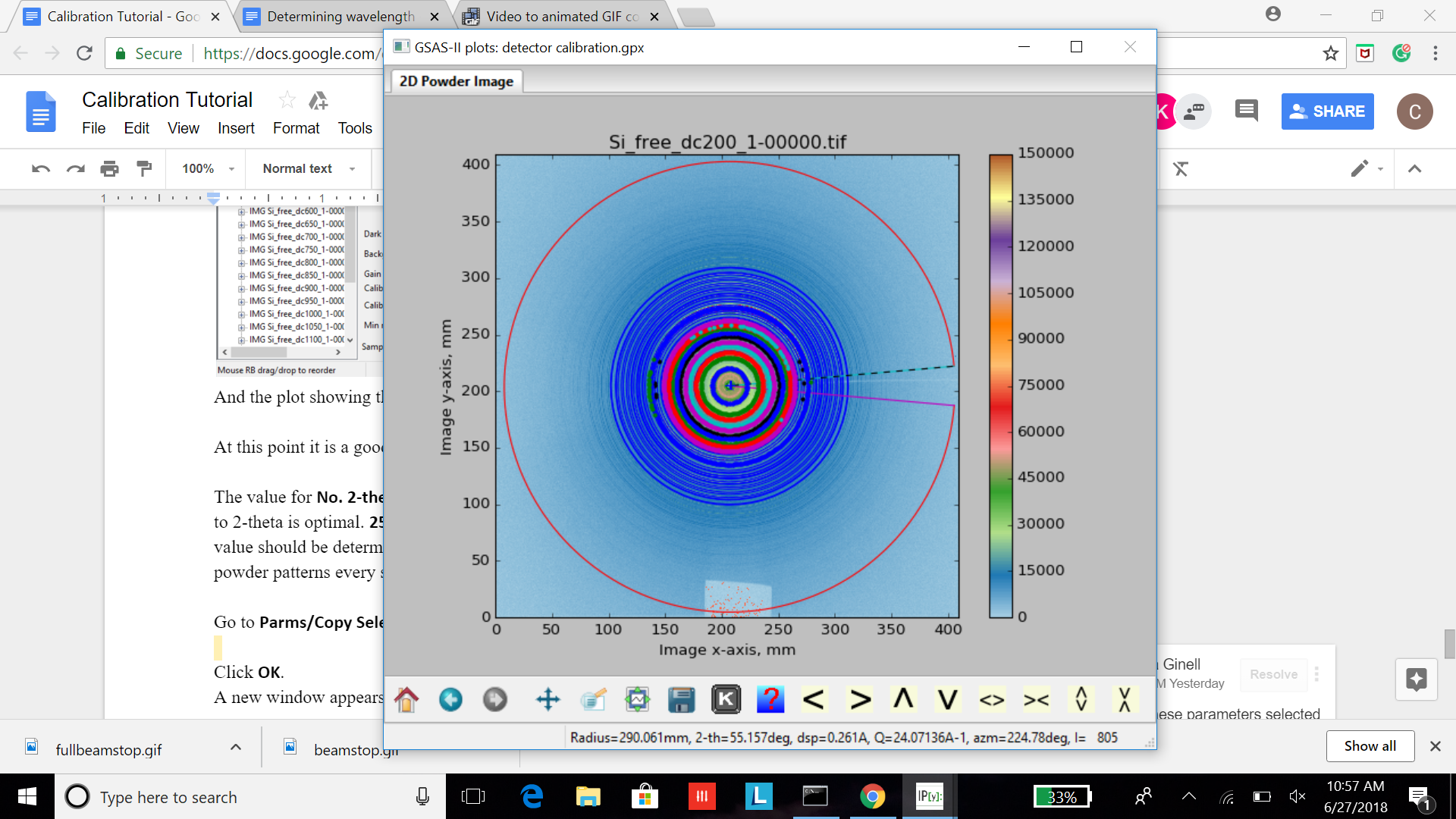
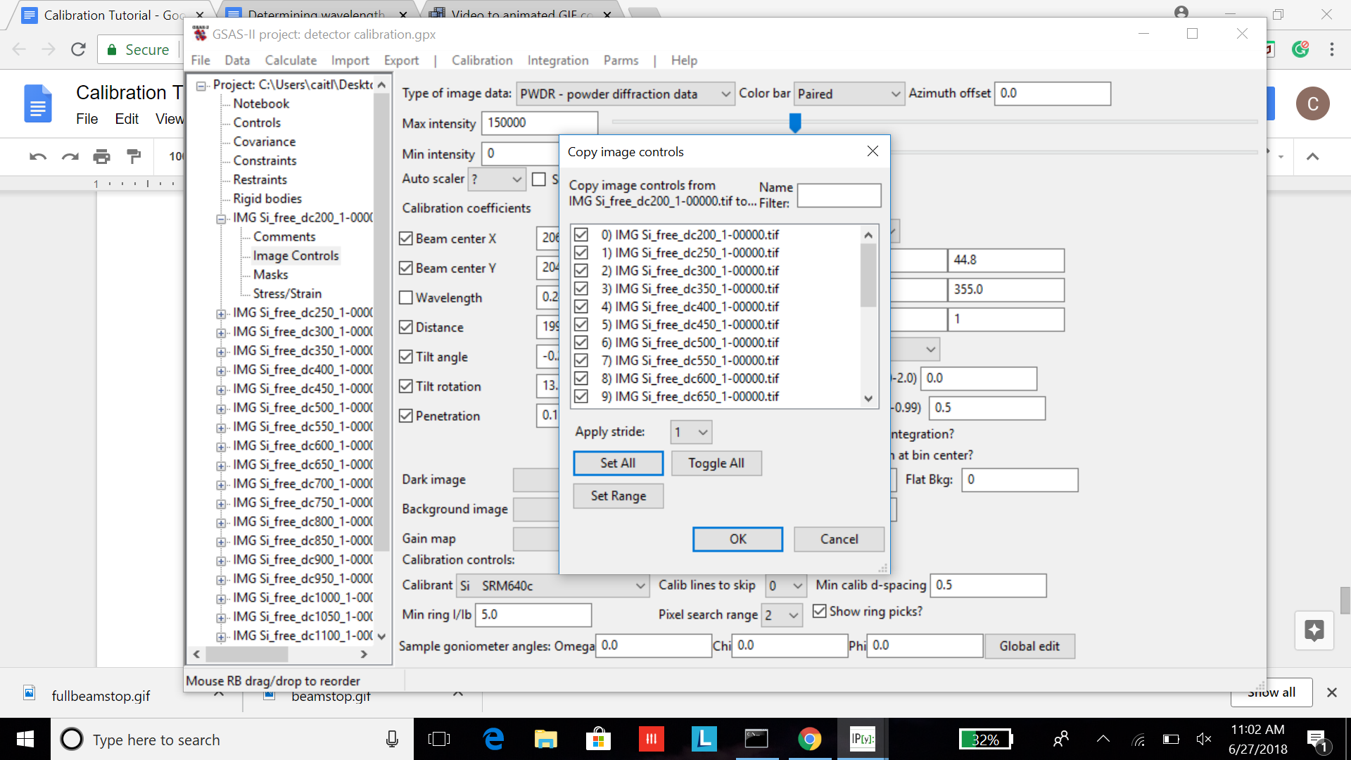
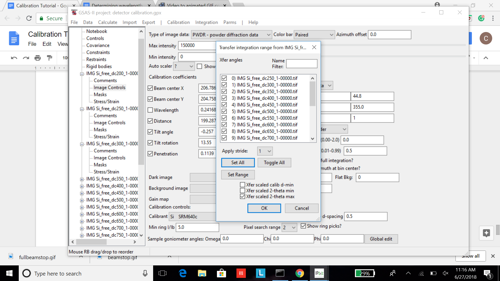
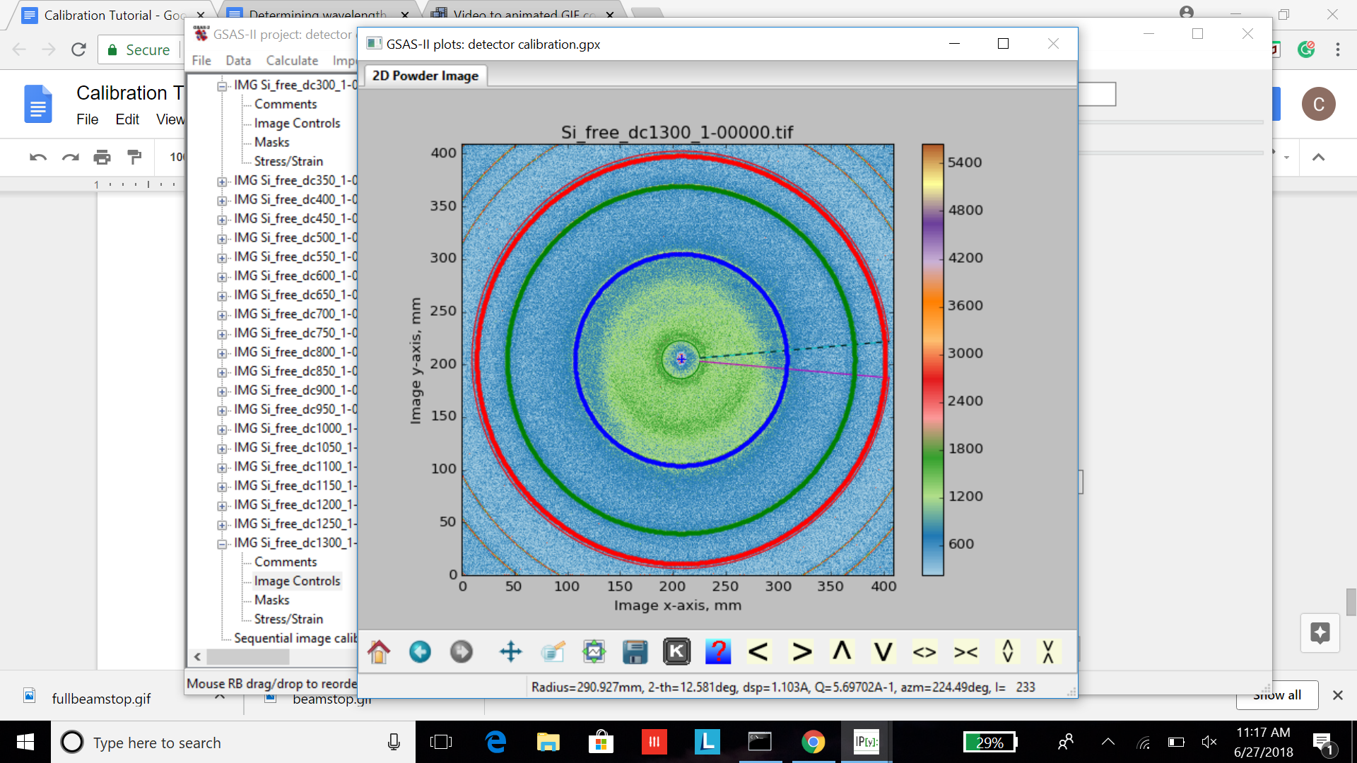
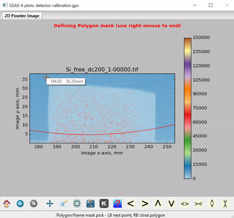
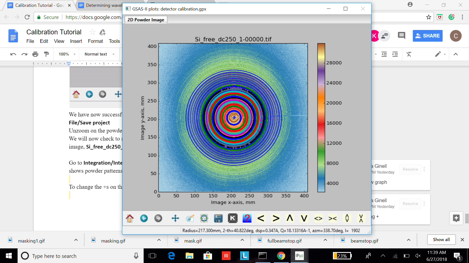
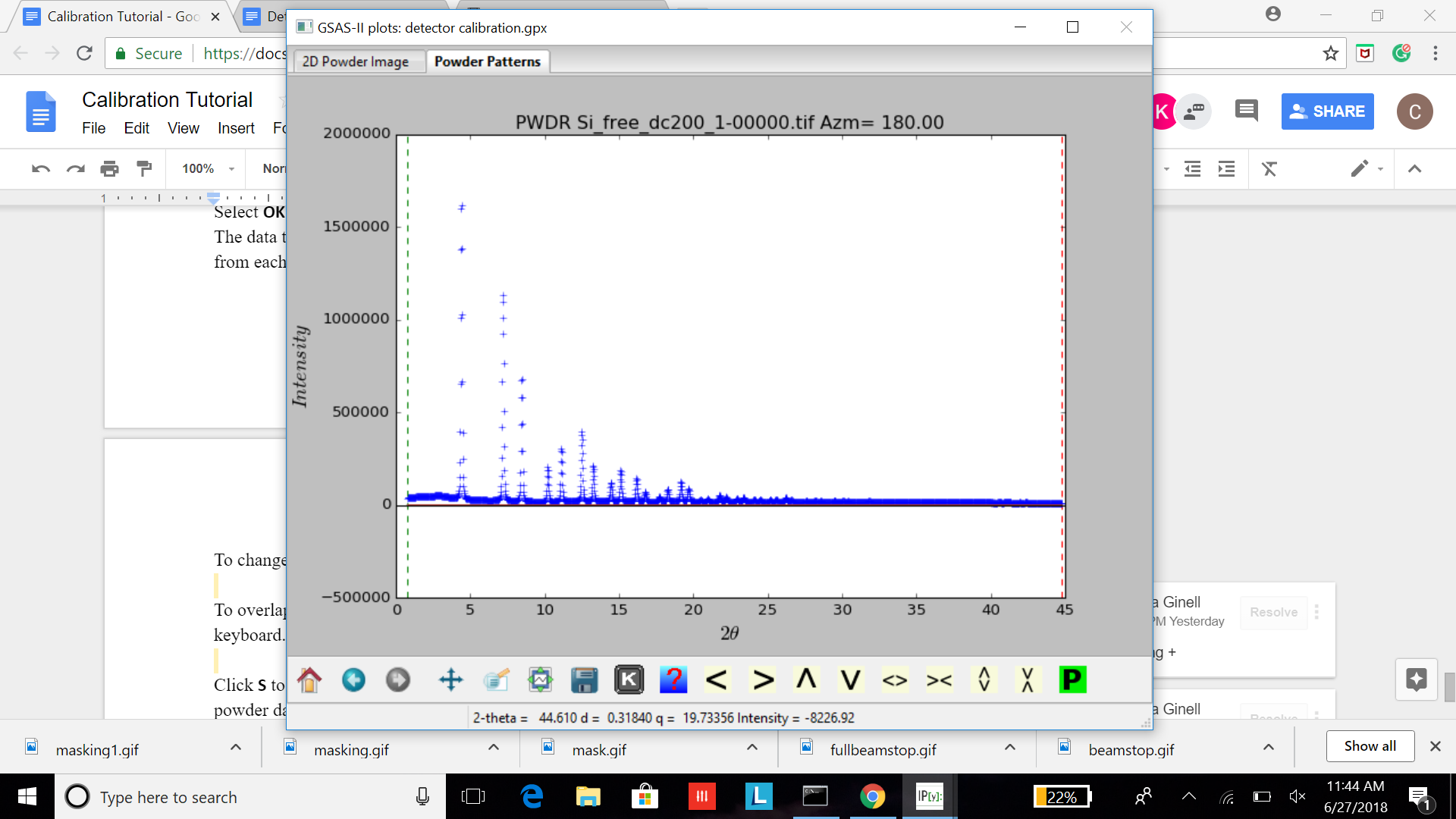
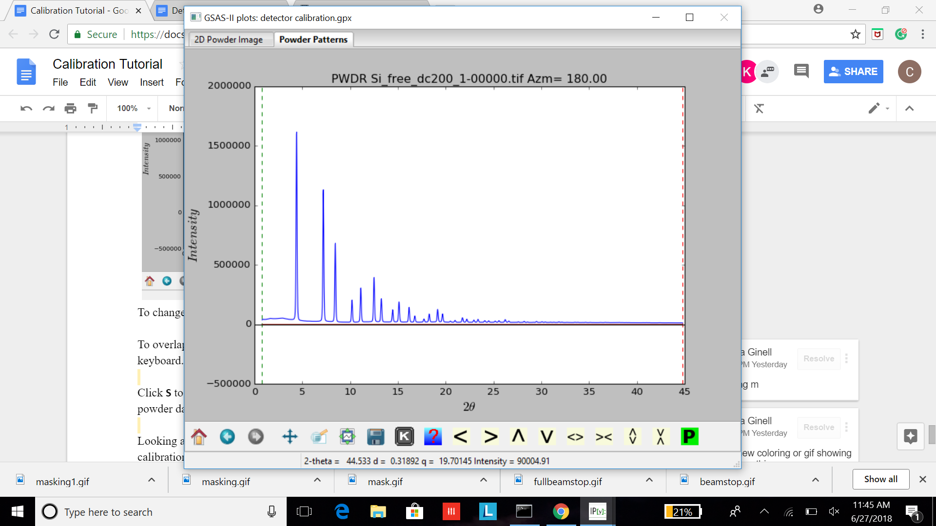
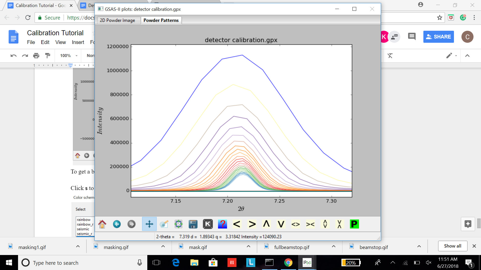
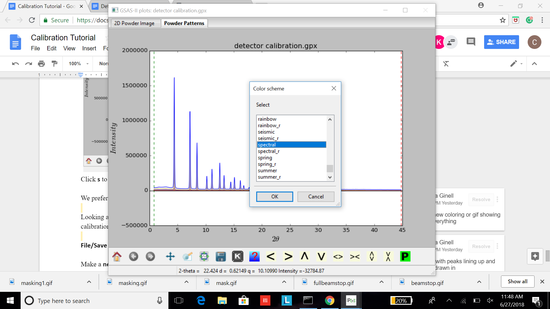
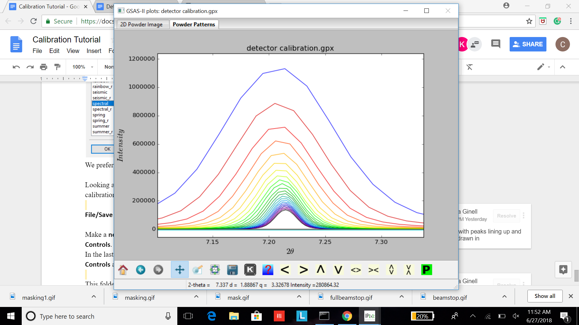
Before stating this, complete the previous tutorial, Area Detector Calibration with Multiple Distances, part 1: Determine Wavelength before beginning this, if you have not done so already. Create a copy of the project to use for calibration by using File/Save project as... to save it under name Silicon_Calibration

Step 1: Finding Average Difference Between Set Distance and Calibrated Distance

Go to Image Controls for IMG Si_free_dc200_1-00000.tif, and change wavelength to 0.241689 as determined in part 1. Uncheck wavelength, and check Distance. We are doing this because we now have a calibrated wavelength, and we want to calibrate the detector distances. The Image Controls should look like this:

In the Image Controls tab for IMG Si_free_dc200_1-00000.tif, do Calibrate/Recalibrate. Keep doing this until penetration (under Calibration coefficients) is constant. Usually recalibrating 3 times will suffice. Our penetration value converged to 0.1139.

The parameters have been adjusted because of recalibration. We want to copy these new parameters to the rest of the images. Go to Parms/Copy Selected. A window will appear like the one below:

Scroll down and select varyList (28) and wavelength (29). Take notice of what parameters are noted as true and false, such as ‘dist’: True, and ‘wave’: False’, these are what will be refined.

Click OK. A new screen will appear. Select Set All to select all images

 and click OK.

Scroll to the bottom of the Data Tree and go to Image Controls for the last image, IMG Si_free_dc1300_1-00000.tif. All of the Image Control parameters set for the first image have been copied to the rest of the images.

Do Calibrate/Recalibrate All/Set All. This recalibration finds the offset of between the set distance and actual distance. The amount of time that recalibrating takes is dependant on the number of pixels. So if there are a large number of pixels for that particular image, then recalibrating will take longer to complete. After the calibration, go to the table under the Sequential image calibration results tab in the GSAS data tree.

From this table we see a column for the calibrated distance (dist) and set distance (setdist) that was recorded when the data was being collected. Although the values are similar, there are slight differences for each image. We will now set up an equation to find the differences between the dist and setdist values.

In the GSAS-II Data Tree, go to Sequential image calibration results/Pseudo Vars/Add formula. A popup window will appear.

Type in the equation a-b next to New PseudoVar= and press Validate. The popup window change and allow you to enter variable types.

Set the a variable as global and a drop down bar will appear

Select dist Global dist. Next, set the b variable as global as well and another drop down menu will appear.

Select setdist Global setdist. Then press OK. A new column called a-b will now appear in the table under Sequential image calibration results.

Double click on the new column: a-b so it is highlighted.

Next, go to the graph called sequential refinement in the plot window.

Click K (at the bottom of the screen)/Select x-axis/setdist. Now the x axis is the set distance.

Next we want to calculate the average. In a perfect world, the graph should be constant at 0 with no error, but at very close and very far distances this is not possible. Select the a-b column once again. Go to columns/rows/compute average. Look at the terminal window.

In the terminal window, we can see the calculated average of -0.123759 and magnitude of +/- 0.287854 for error. The error in this case, is very high (around 0.3).

Notice that the first and last few images are the least accurate because they are either too close or too far away from the detector to gather an accurate reading.

Therefore, go to Sequential image calibration results and unclick image use for images 200-400 and 1050-1300. The table should look like the following:

To calculate the average again, select the a-b column again by double clicking on the column header then go to Columns/Rows/Compute average. The terminal window will show:

 The magnitude of error of +/- 0.045307 is much smaller and more desirable. Therefore we feel more confident saying that the average distance between set distance and calibrated distance is -0.167927

Step 2: Integrating the Calibrated Data

This next step involves integration of the data. Go to Image Controls for the first image, Si_free_dc200_1-00000.tif and then go to the GSAS-II plot window. Select the tab with the powder data rings. Notice shadowed regions from the beamstop and pin diode. In the final integration, we do not want to use these areas, so we will work on excluding these from the integration.

In the GSAS-II data tree, go to Image Controls for the first image, Si_free_dc200_1-00000.tif. We will be working in the Integration coefficients area. Click Show integration limits?. The plot should show the area that is to be integrated.

Zoom in on the beamstop (bullseye of rings) so we can make sure to exclude this from our final integration.

Change the inner 2-theta to a smaller value of 0.8 to only exclude the small beamstop in the middle and not the surrounding data.

Click the home button to see all the rings. Drag the mouse to the rights side of the image. As the mouse moves to the right, 2-theta changes at the bottom of the screen. Note the outer 2-theta value when the mouse stops at the edge of the screen.

Type this value (we used 44.80) into the Outer 2-theta box. Check the Do full integration? Box.

The image controls screen should look like this:

And the plot showing the integration limits should look like:

As we can see from the image, the inner and outer angles that we entered gave us a good integration area around the powder rings.

At this point, we are going to cut out the beamstop, which yields poor intensity data. So, remove the Do full integration? Box.

To exclude the beamstop we will adjust the start/end azimuth degrees. Make the Start azimuth 5, and End azimuth either 355 or -5.0 (it does not matter). The image controls window should look like the following:

And the plot showing the integration limits should look like the following:

As we can see, the beamstop will now be excluded from our integration of the data.

At this point it is a good idea to use Save project.

The value for No. 2-theta depends on the number of pixels in the detector. A 1:1 ratio of pixels to No. 2-theta is optimal. 2250 for our No. 2-theta value works with our detector size and pixels so we will leave it as is. However, know that that value should be determined by the detector size and number of pixels. Azimuth bins finds powder patterns every so many degrees. We have it set at 1.

Go to Parms/Copy Selected and select fullintegrate = false (12), IOtth (15), LRazimuth (16), and outAzimuths (18), .

Click OK.

A new window appears. Click Set All 

Then select OK.

Now go to the Image Controls of the last image, Si_free_dc1300_1-00000.tif. Check Show integration limits? and change the auto scaler to 95%.

As we can see, the 2-theta max angle is off for this image.

To fix this, go to the first image, Si_free_dc200_1-00000.tif, then Image Controls, and finally Parms/Xfer angles. Select Xfer scaled 2-theta max and Set All.

Click OK. This fixes the maximum angle on all of the images based off the scale we set to the first image. The minimum angle does not change. Here are the correct integration limits for the “1300” image:

Save project once again.

We have changed the parameters so that GSAS-II does not integrate the beamstop. We will now use a mask to exclude the pin diode. Go back to the first image once again, Si_free_dc200_1-00000.tif, but this time go to the Masks section under the data tree. Zoom in on the pin diode in the GSAS-II plots window.

Do Operations/Create new/Polygon mask. Go to the plot window. Pan the mouse around the pin diode to create a quadrilateral surrounding the light area (pin diode). Click on the plot for each corner of the mask. Lines will be drawn in to connect the corners. Create the mask so that it borders the pin diode.

We have successfully masked the pin diode so it will not be included in our integration.

File/Save project.

Unzoom on the 2D powder image (can be done by clicking the home button).

We will now check to make sure there is no pin diode in any of the other images. Go to the 2nd image, Si_free_dc250_1-00000.tif/Image Controls. Change the Autoscale to 95%.

As we can see, the pin diode did not show up in this image or any of the following. Therefore, we do not need to do any more masking.

Go to Integration/Integrate all. In the pop-up window, select Set All.

Select OK.

The data tree now shows PWDR files for each image. The new graphs show the powder patterns from each of the integrations and should look something like this:

In order to show continuous lines on the graph, press the + key on your keyboard.

To overlap all the cells onto one graph, click on the K/toggle multidata plot or click m on your keyboard.

To get a better view of the overlap of data, we zoomed in on the second peak from the left.

Click s to show a choice of color schemes.

We prefer spectral (lowercase option). Choose the desired scheme then press OK.

We can tell this is a very accurate calibration because all of the peaks from each image line up very well.

File/Save project.

We will now save this calibration data into a folder on your computer so it can be used at anytime as a calibrant for measuring an unknown substance.

Make a new folder on your computer (wherever you want to store these calibration files) and call it Image Controls.

In any image, go to Image Controls, then go to Parms/Save Multiple Controls and a popup window will appear. Click Set All.

Then press OK.

Click on the newly made folder (Image Controls) where you want to store these files and click Select Folder.

This folder will now contain all the image controls and parameters to be used for future measurements.

We have now finished the calibration process. Based on the calibration, a user can access the image controls folder and obtain information about the calibrated data. This will be important for accurate future data collection. To use these saved parameters, open a new project and select Parms/Load Multiple Controls and then this will load all parameters.