In this tutorial you will use a standard with a known lattice parameter (silicon) to determine the wavelength of the X-ray beam without precise knowledge of the sample-to-detector distance. This is done for APS beamline 17-BM-B by collecting diffraction data with multiple detector distances, where the relative placement of the detectors is known to some degree. Here 23 images with approximate placements ranging from 200 to 1300 mm from the sample. First the x-ray wavelength is determined and then in a subsequent tutorial that wavelength is used to calibrate the actual detector placements.

Note that menu entries are listed in bold face below as Help/About GSAS-II, which lists first the name of the menu (here Help) and second the name of the entry in the menu (here About GSAS-II). Bold text is also used to highlight actions, such as clicking on a control in the GSAS-II graphical interface.

If you have not done so already, start GSAS-II or start a new project.

Step 1: Load data

First do Import/Image/from TIF image file,  select all images; then press Open to read all of them. The GSAS-II data tree window will show entries for 23 images and will expand the last one. If the files have not been downloaded with this tutorial, they can be found here: https://subversion.xray.aps.anl.gov/pyGSAS/Tutorials/DeterminingWavelength/data/ .

Step 2: Calibrating the Wavelength: First Image

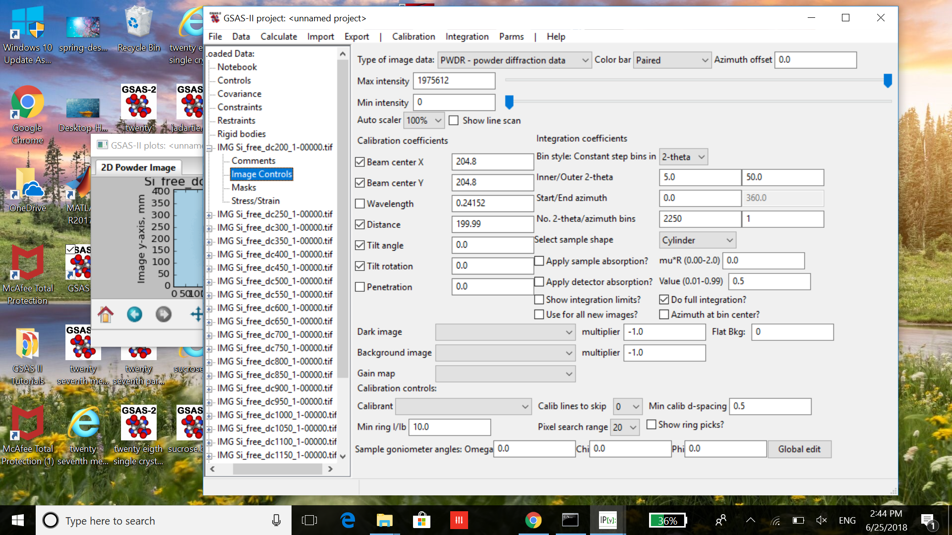
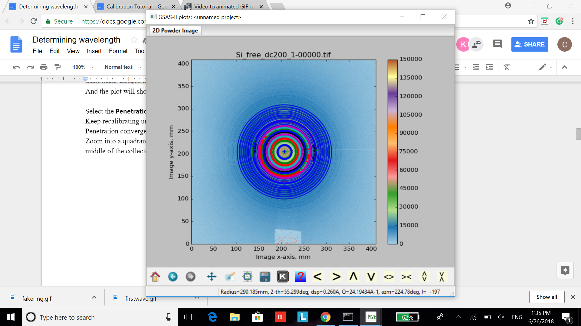
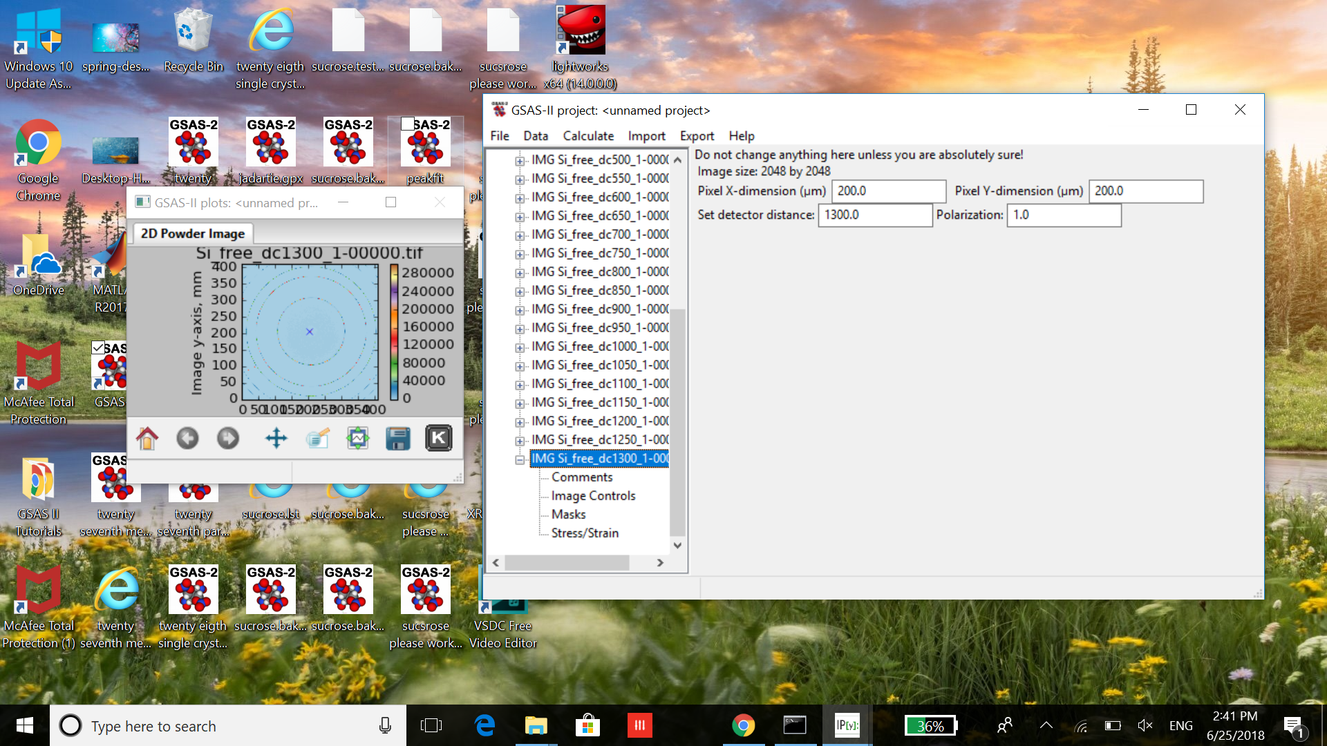
First select the IMG Si_free_dc200_1-00000.tif entry from the tree (the first in the tree) and expand it (press the + box); then select Image controls. The data window (Image Controls) will show the default settings.

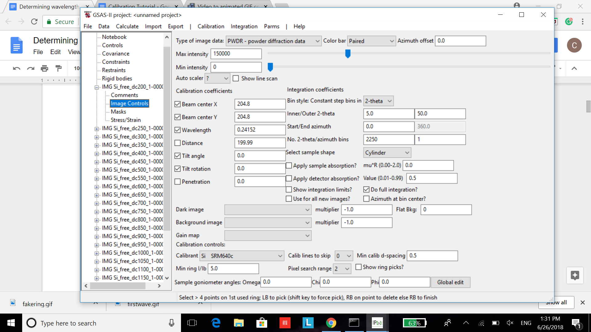
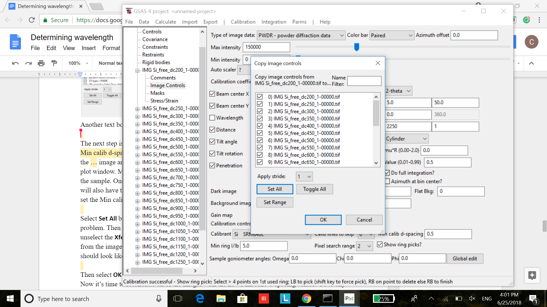
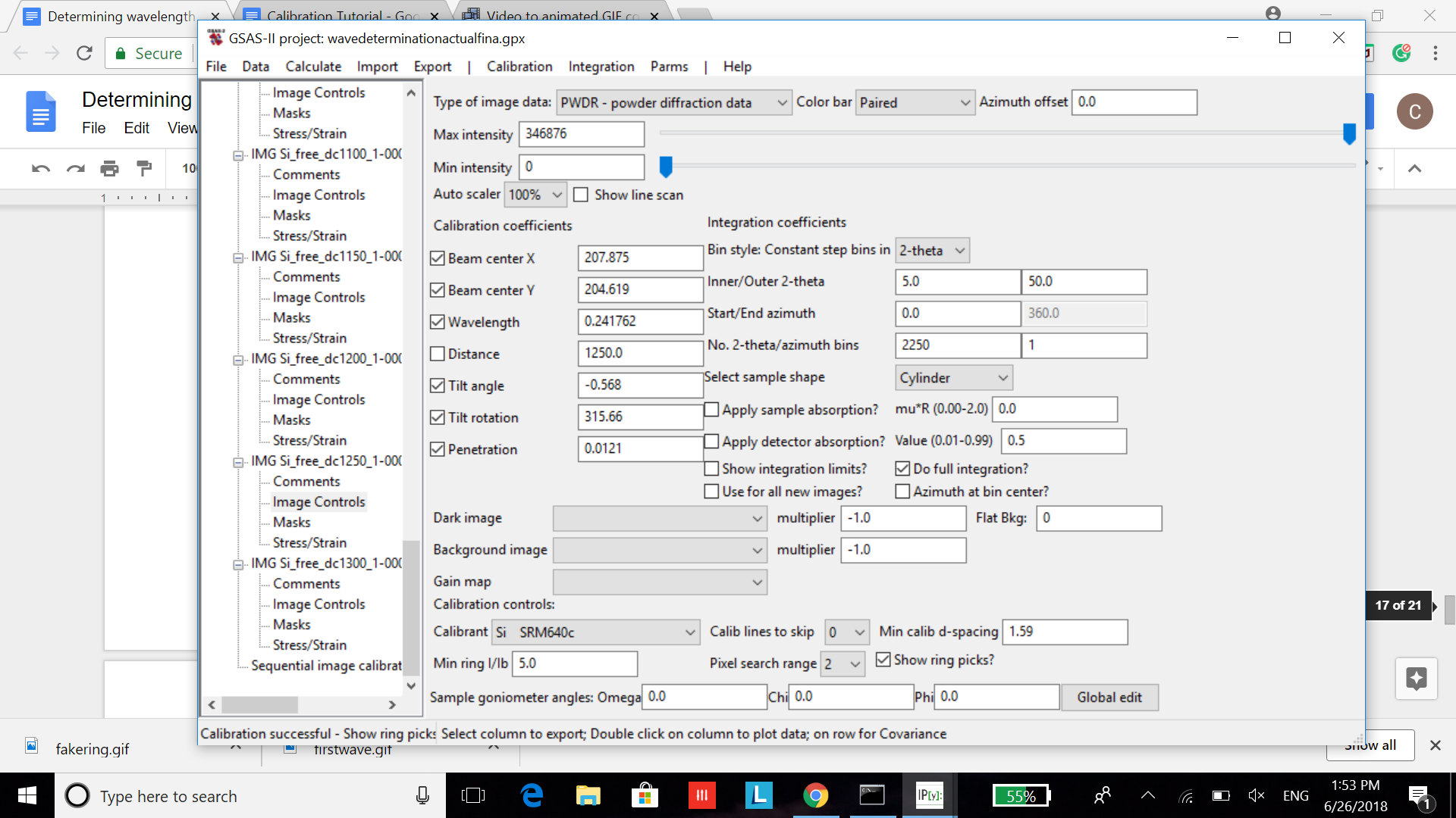
Select the Calibrant (near bottom of window) as Si SRM640c. Check the box next to Wavelength and uncheck the box next to Distance. We are doing this because we will initially treat the reported setting distance to be correct, and will use that to determine the unknown wavelength. You should move the Max intensity slider to near the middle of the range (we chose 150,000) – that will improve the image. Change Min calib d-spacing to 0.5, Min ring l/lb to 5.0, Calib lines to skip to 0, and Pixel search range to 2. When done the Image controls window should look like:

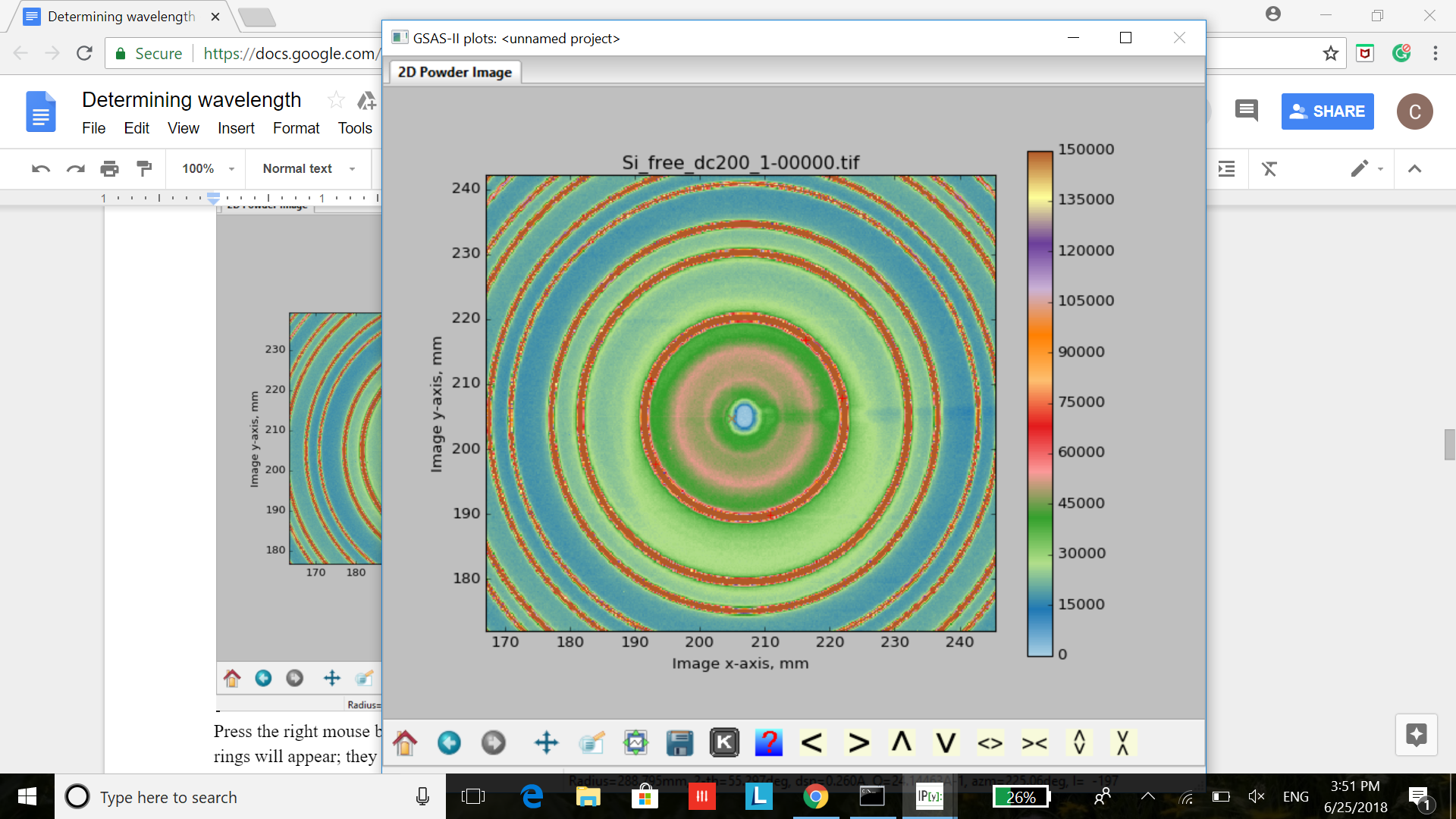
Next select Calibration/Calibrate from the Image Controls menu; a bit of instruction will appear on the status line of this window. Zoom in so that the innermost rings are clear. Select 5 points on the innermost ring (arrowed above); a small red cross will appear at each selection point (may have to reload page for crosses to show up).

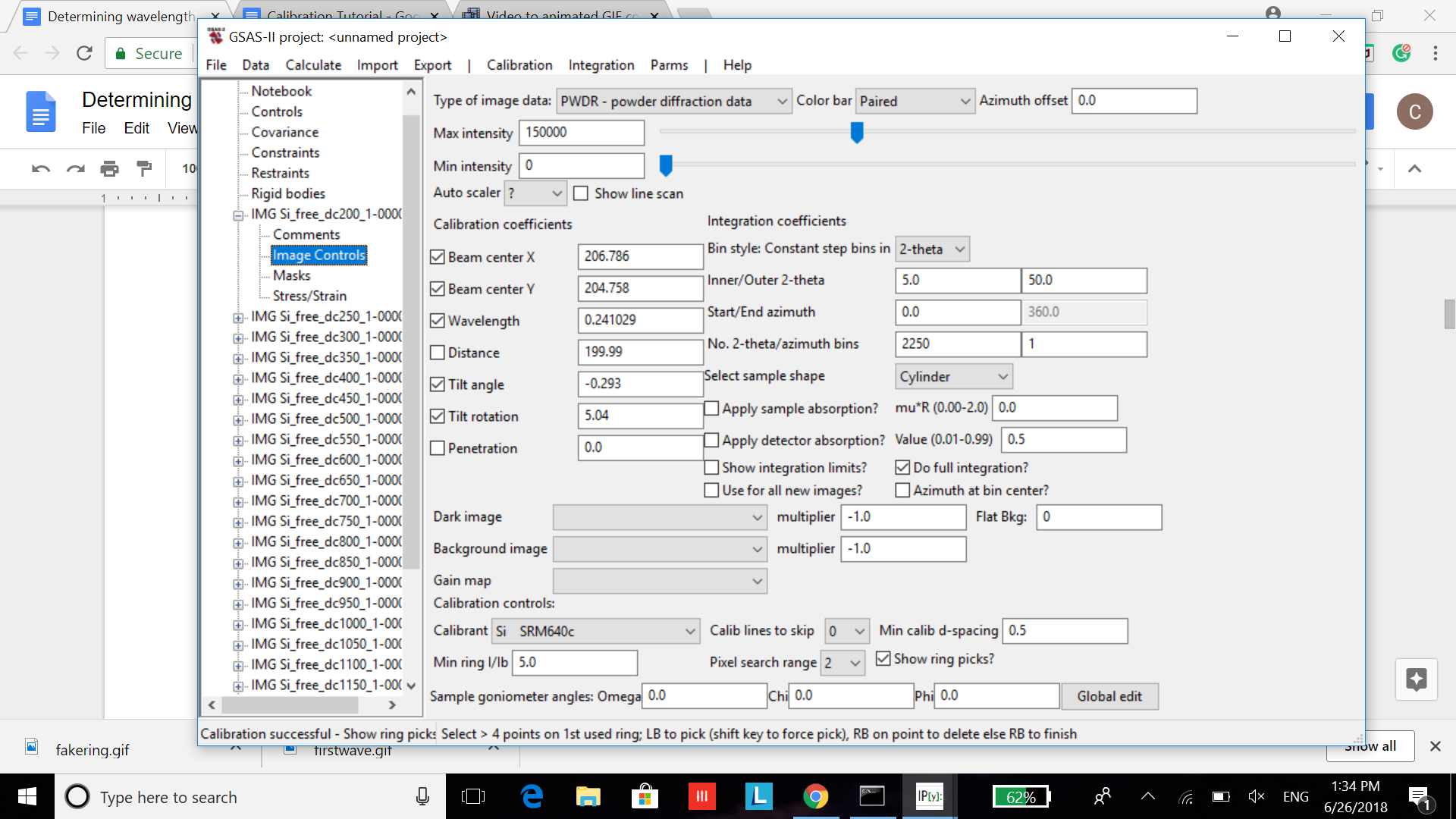
Press the right mouse button to finish; calibration will proceed. A sequence of concentric red rings will appear; they will switch to blue when calibration is finished. Select Show ring picks (near bottom right of Image Controls window). The Image Controls window will show the results of the calibration

And the plot will show the rings used in the calibration calculations.

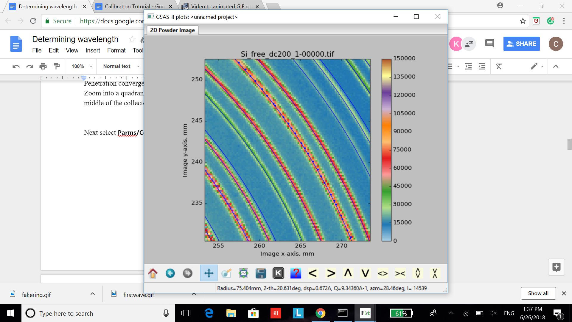
We can improve the fit by refining a penetration correction; select the Penetration  and then we can recalibrate. Select Calibration/Recalibrate. Keep recalibrating until the penetration value converges to a constant value. The value that our Penetration converged to 0.1433. Zoom into a quadrant of the rings and check to make sure the blue calibration lines are towards the middle of the rings in the collected data

Step 3: Calibrating all Images

Since the single-image calibration looks good, it is time to copy these parameters onto the rest of the images.

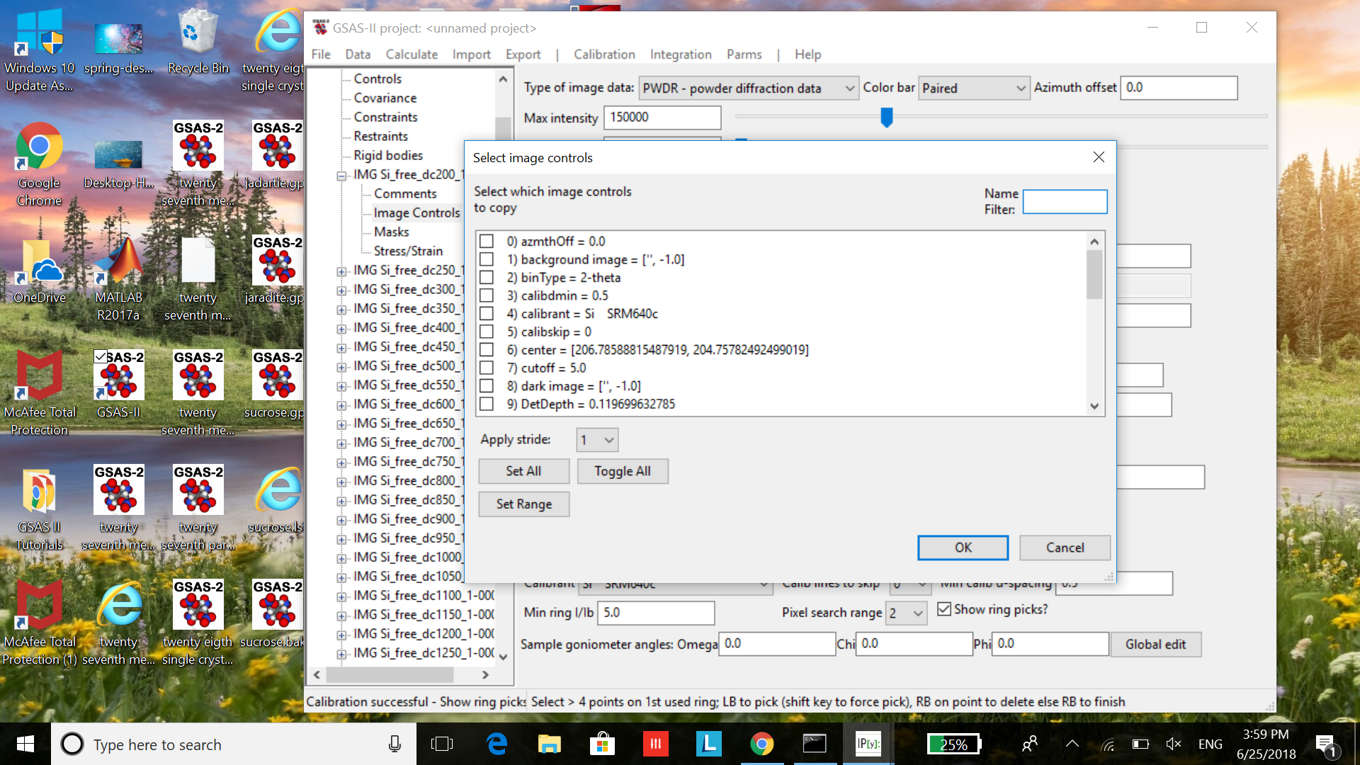
Next select Parms/Copy Selected. A text box like this will pop up:

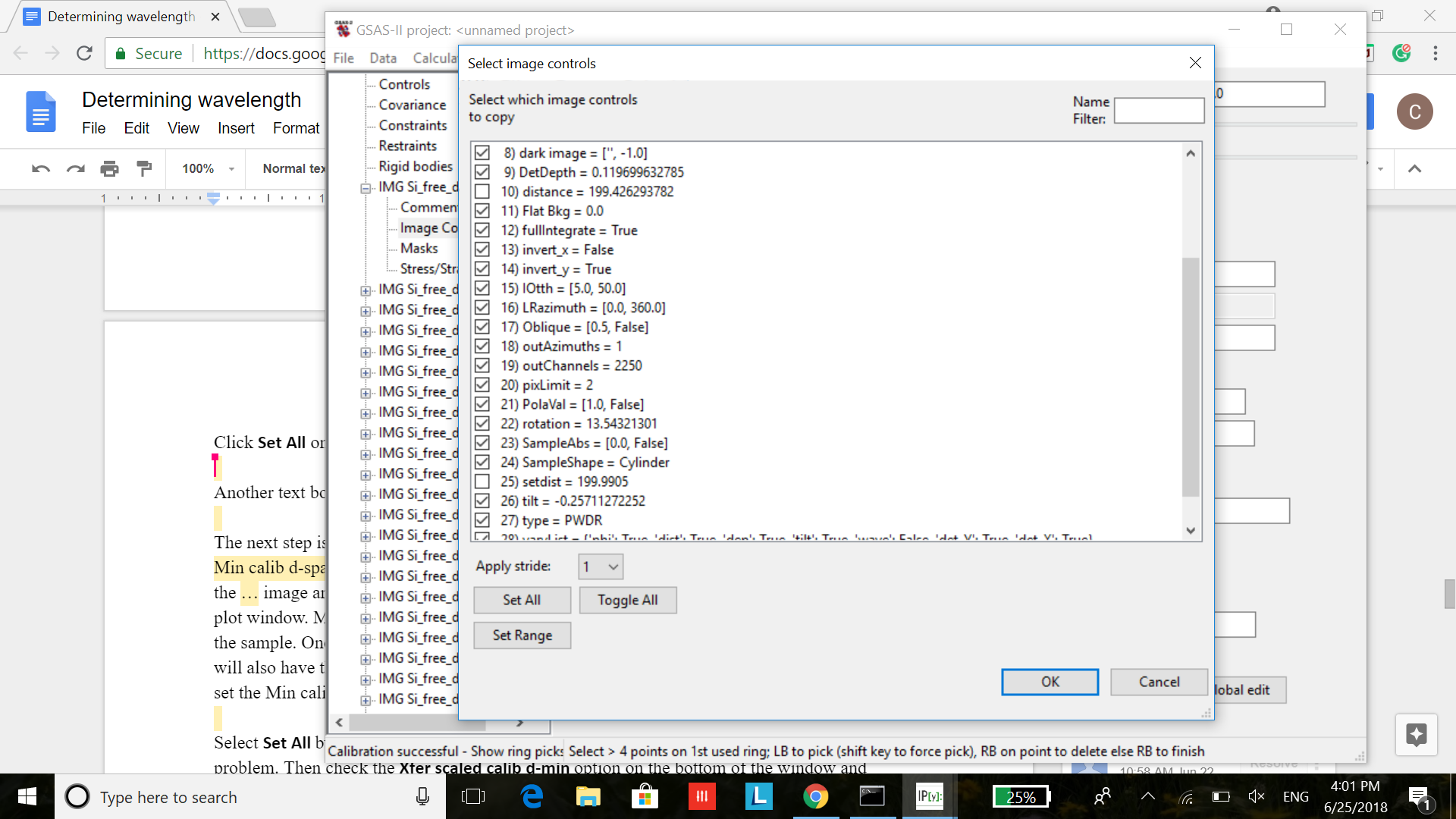
Click Set All on the bottom then go back and unselect both distance (#11) and setdist (#26), as below, then press OK. We want to copy all parameters except for the distances because they differ for each image.

Another dialog box will appear for selection of the images to copy these parameters to, hit Set All and press OK

Next select Calibration/Recalibrate all to recalibrate all images with the new parameters.

Do File/Save project as... and name it Wavelength_Determination. This will create a copy of the project to use for calibration.

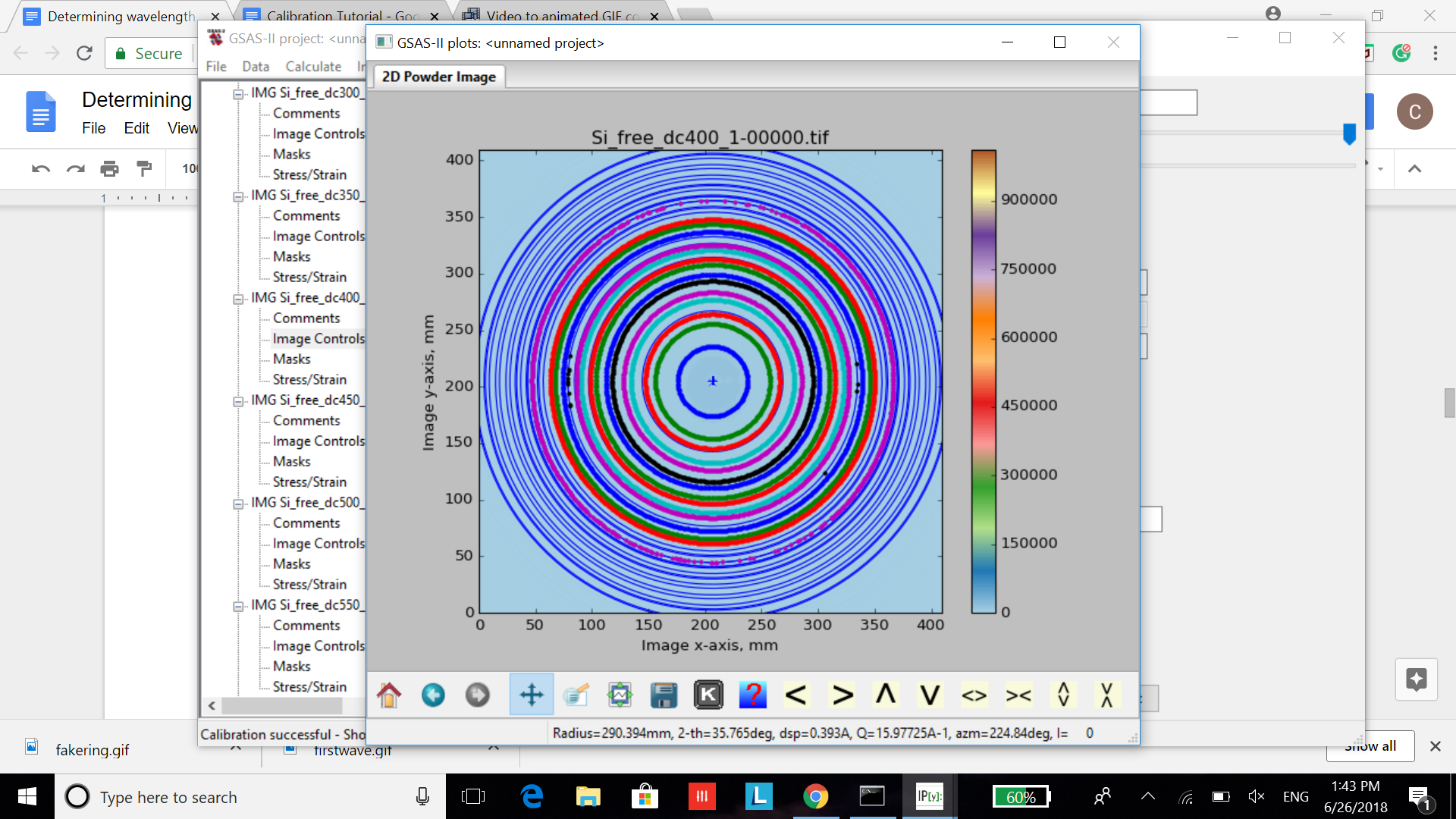
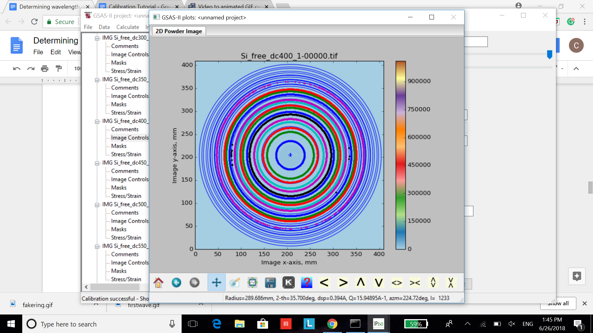
The next step is to check to make sure the Min calib d-spacing setting value ensures that only full rings are used in each calibration. The Min calib d-spacing restrict the set of reflections to be used. To do this, start at the Image Controls for the first image and then go in increasing order through the images until you find one where the outer rings are cut off. For us, the first image with rings cut off is IMG Si_free_dc400_1-00000.tif, as below.

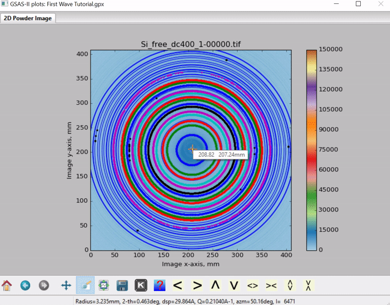
Start with your cursor in the center of the rings and then pan your mouse over to the right edge. Watch the Min calib d-spacing decrease as you continue to move the mouse to the right.

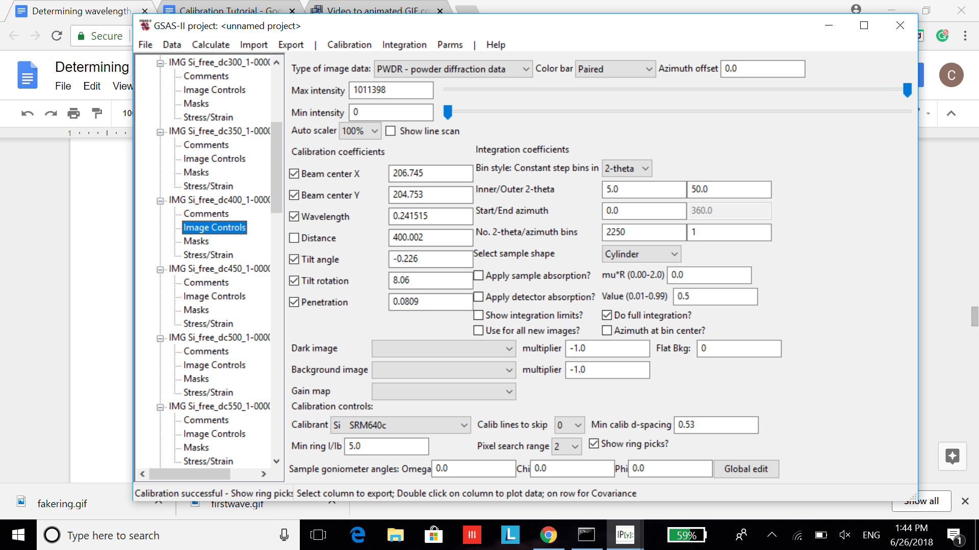
Look at the dsp value at the bottom of the plot window. Look at the value when the cursor is on the edge. That will be the new Min calib d-spacing. The default value of 0.50 is allowing the outer rings to be cut off.  We then looked at what the dsp value was when the cursor was on the edge of the image. Here it is 0.529, so we went to image controls  for image IMG Si_free_dc400_1-00000.tif and changed Min calib d-spacing to 0.53.

Then select Calibration/Recalibrate and the image should now have all the rings intact.

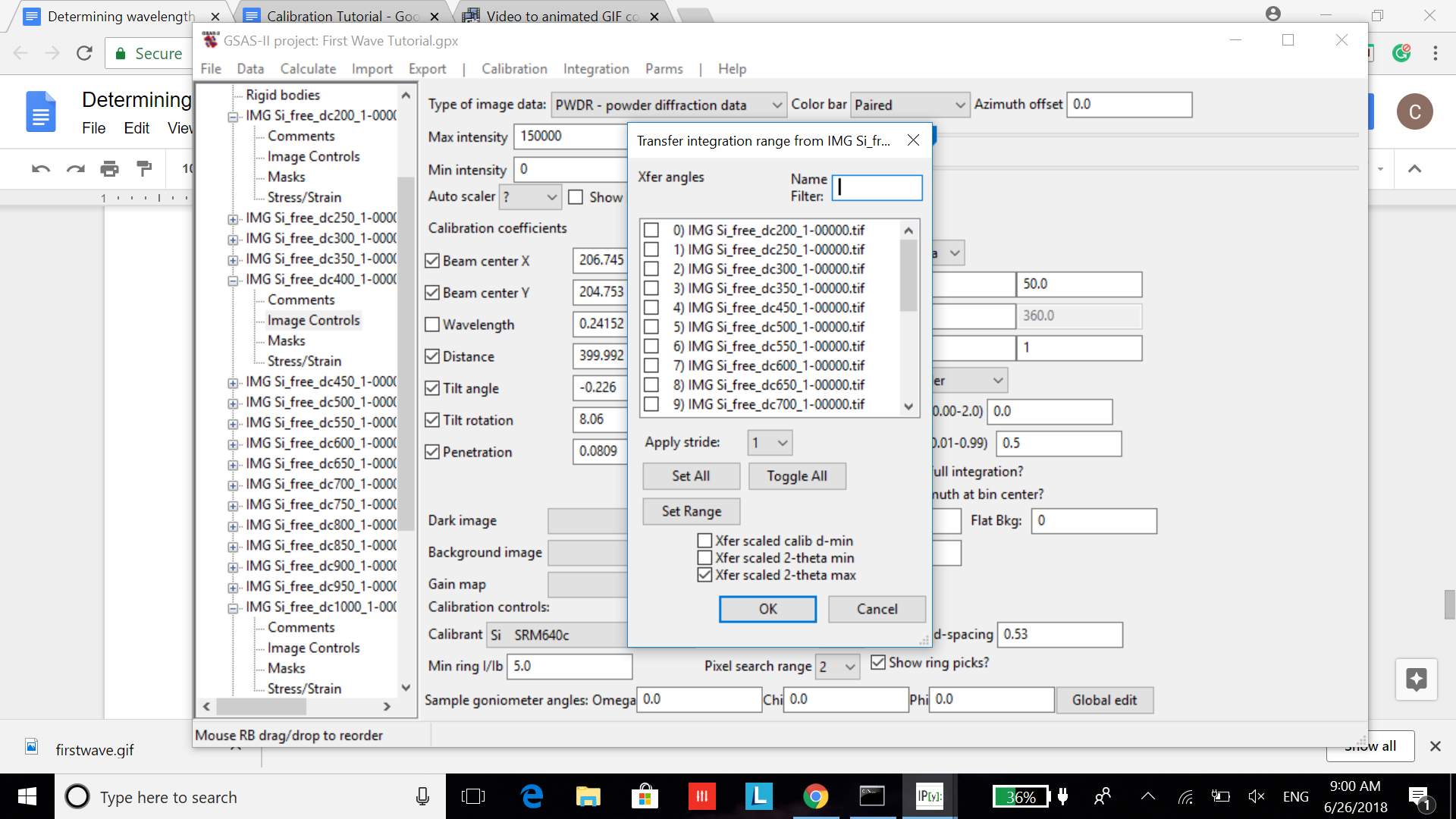
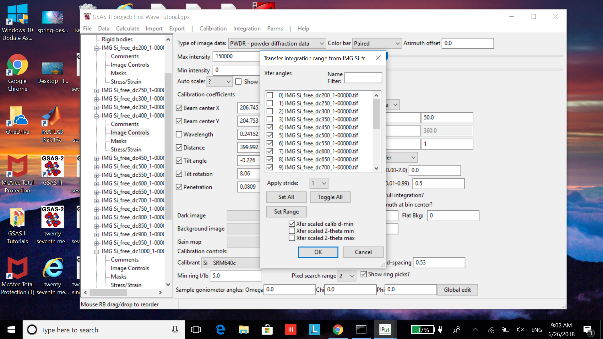
After you fix the first image where the Min calib d-spacing is off you can fix the rest of the images that also have this problem. To fix this, select image controls for image IMG Si_free_dc400_1-00000.tif. Then select Parms/XFer Angles and a window will pop up.

Select Set All but then unselect all the earlier images that did not have a Min calib d-spacing problem. For us, this was images 200-350. Then select the Xfer scaled calib d-min option on the bottom of the window and unselect the Xfer scaled 2-theta max option. This takes min calibrated d-spacing from the image selected and determines the accurate d-spacing for all other images. The text box should look like the following:

Then select OK and the rest of the Min calib d-spacing will be adjusted for the rest of the images.

Now it’s time to recalibrate all of the images with the new Min calib d-spacing values. Go to any image controls window and select Calibration/Recalibrate all and select Set All.

This will take a bit of time as each image is being recalibrated.

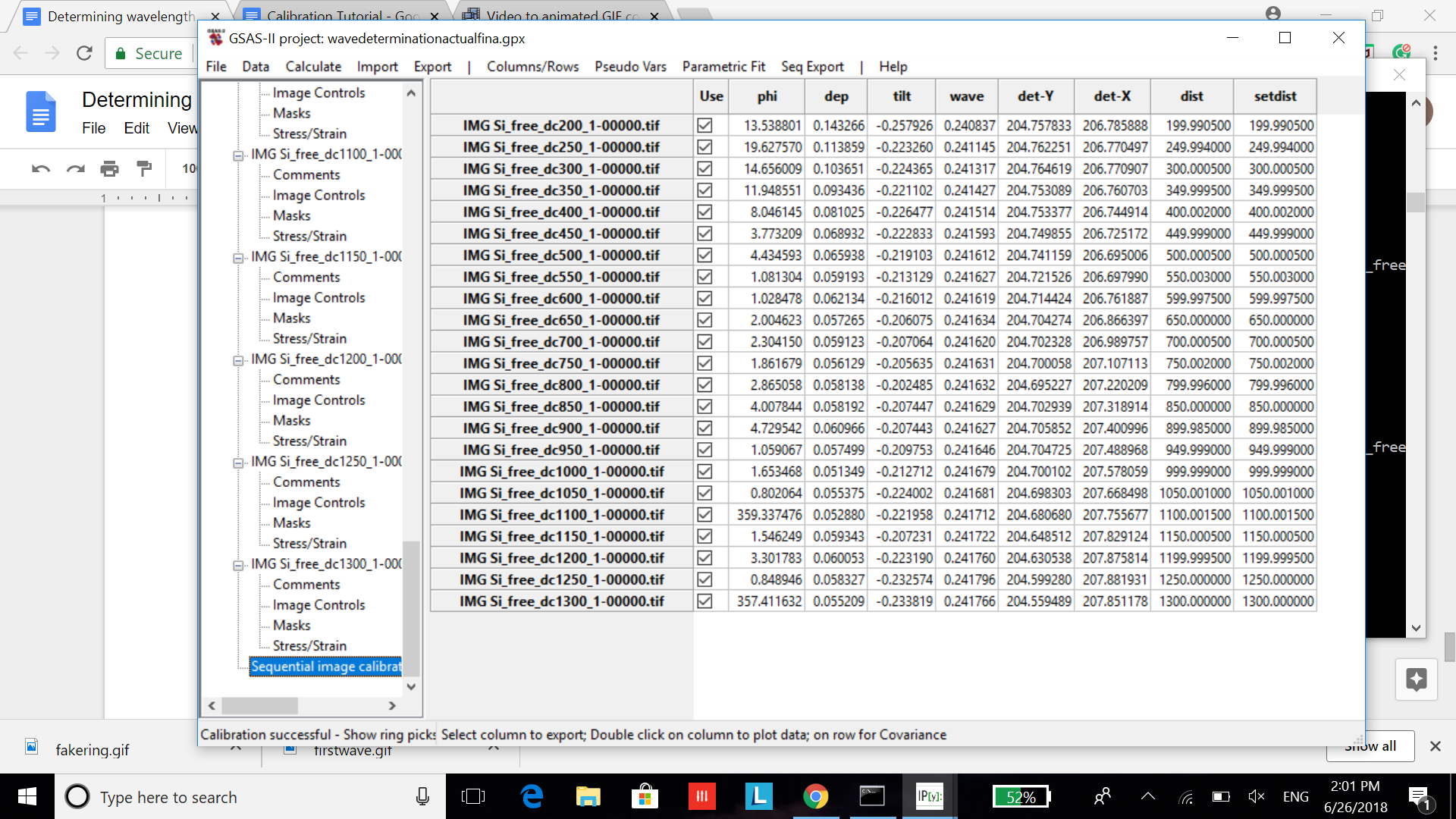
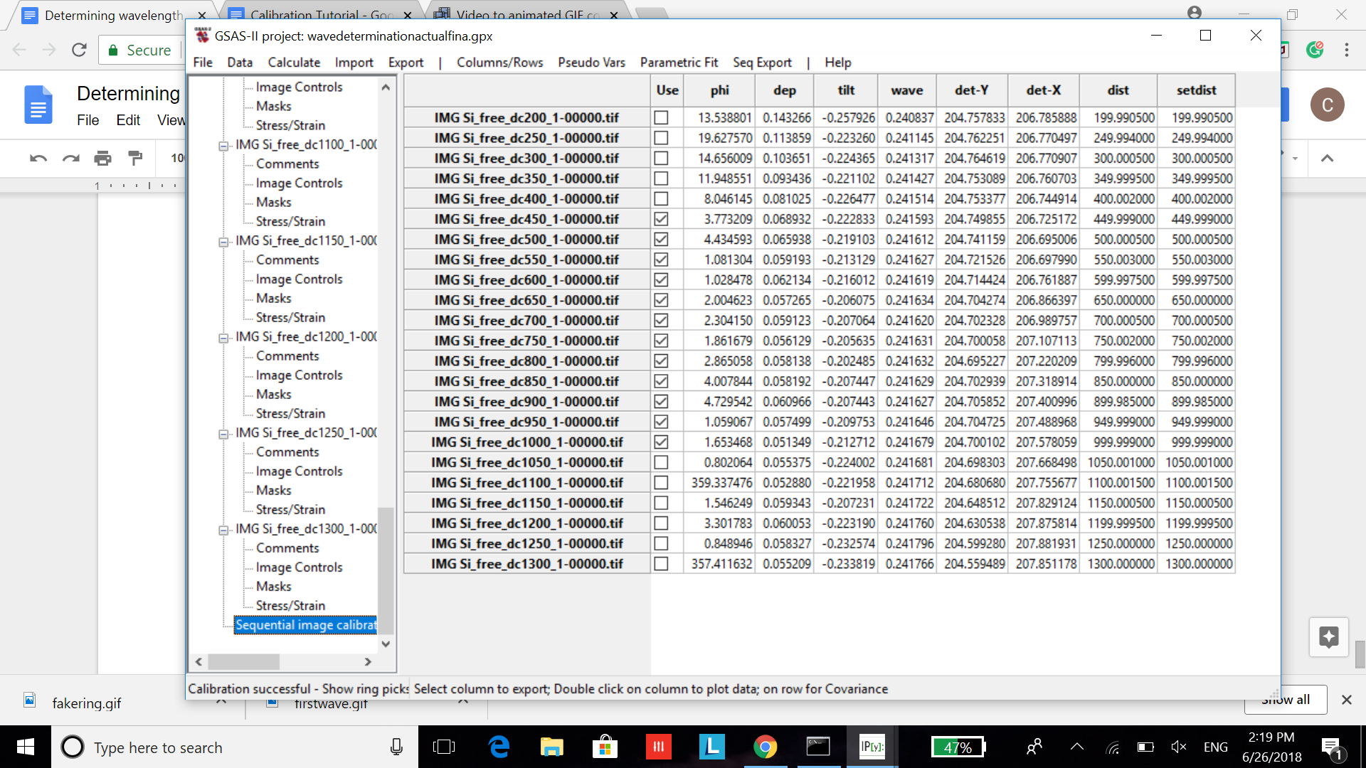
After the recalibration, all the images should only have full intact rings. Once the process is complete go to the bottom of the data tree and select Sequential image calibration results and a table should appear.

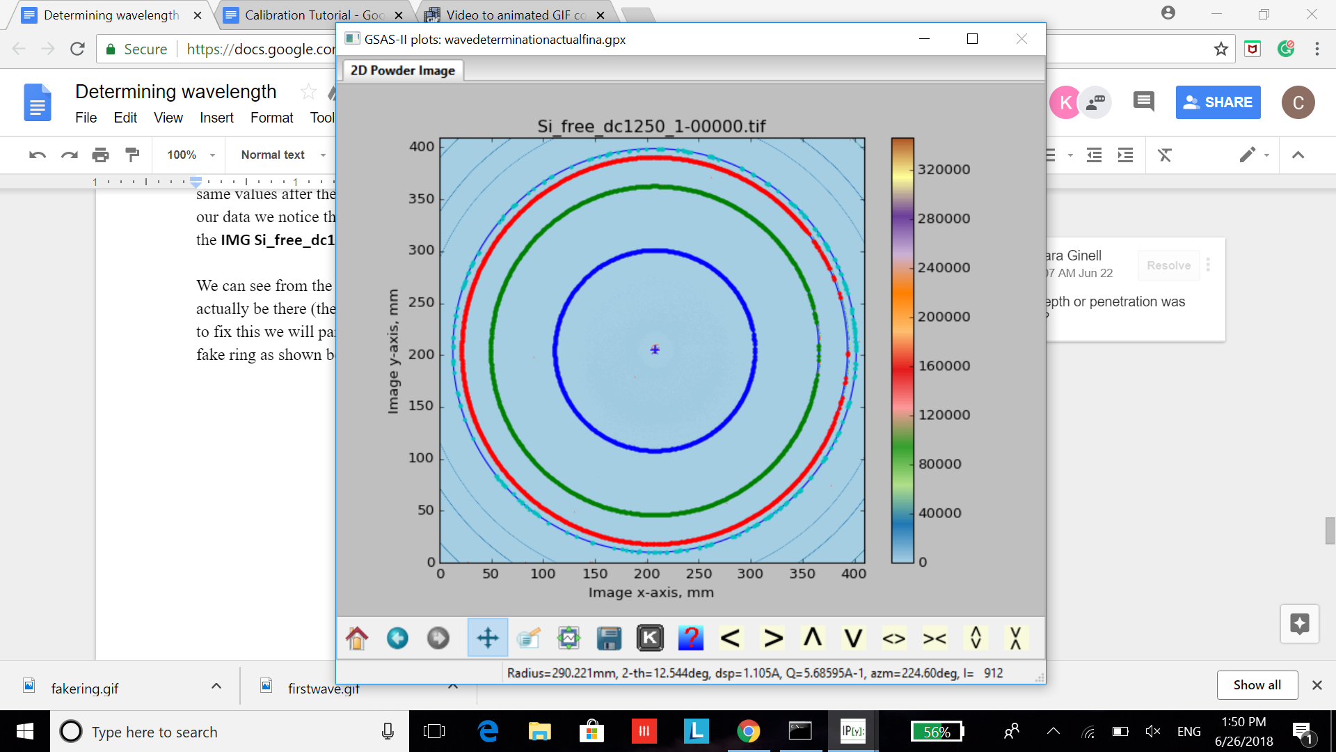
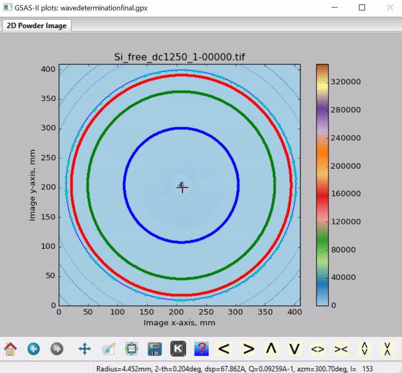
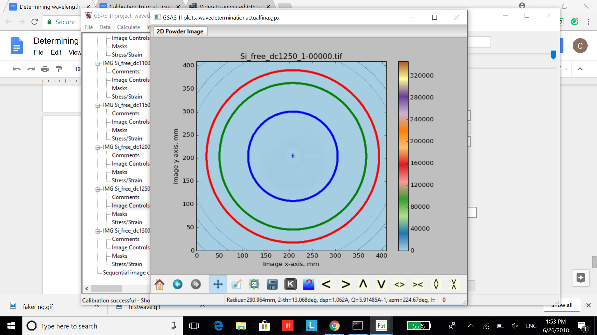
In Sequential Image Calibration results, a table should appear with a column labeled dep containing detector penetration depths (dep). As we look over the table we need to make sure that the detector penetration depths have roughly the same values except for the first few rows (these will be off due to the close distances). As we look at our data we notice that the last few values are inconsistent with the rest. To investigate we select the IMG Si_free_dc1250_1-00000.tif/ Image Controls and view the second to last image.

We can see from the image that there is a fake (or fragmented) fourth ring that should not actually be there (the last “1300” image does not have this issue of the fake fourth ring). In order to fix this we will pan the mouse over to the space in between the last full ring and the fake ring as shown below.

We found a value of the dsp to be 1.592 and changed the Min calib d-spacing to that value under Image controls for the “1250” image.

We then selected Calibration/Recalibrate and our image now excludes the fake fourth ring.

Continue to go through the images in decreasing distance from the detector and check to see whether there is a phantom ring and adjust the Min calib d-spacing accordingly. However once you get to an image where there is another full ring outside of the phantom ring, there is no need to adjust the Min calib d-spacing. We adjusted the Min calib d-spacing value to 1.59 for images IMG Si_free_dc1200_1-00000.tif and IMG Si_free_dc1150_1-00000.tif. The “1100” image had a fifth full ring that we did not want to exclude.

After completing this process select Calibration/Recalibrate all once again. Continue calibrating until the dep values converge. After a few recalibrations, the table under Sequential image calibration results shows our dep values converge the detector distances are further from the sample.

Our new values have improved quite a bit. If the any  detector penetration depth (dep) values are negative then go to Image Controls for the images with negative dep values. You will see that the penetration values for those images are also negative. As this should not be possible, change the value of Penetration to zero and then did Calibration/Recalibrate all once again and the penetration values should become positive. If required, turn off refinement of Penetration with a value of 0.0 if that is the only way to keep the value from becoming negative.

Step 4: Parametric Fit to Find Wavelength

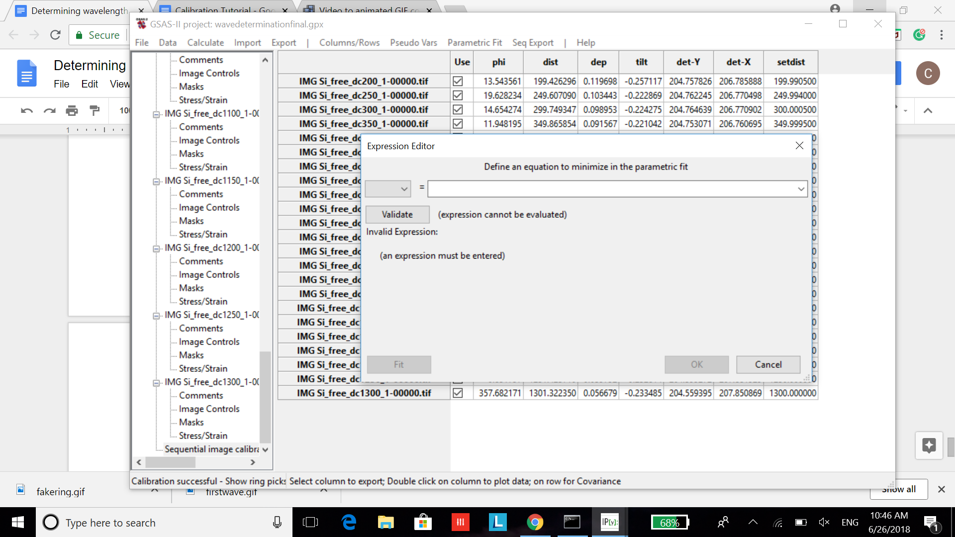
The refinement is giving good calibration values so it’s now time to graph our values. Under the Sequential image calibration results tab in the data tree select Parametric Fit/Add equation and a new window should popup.

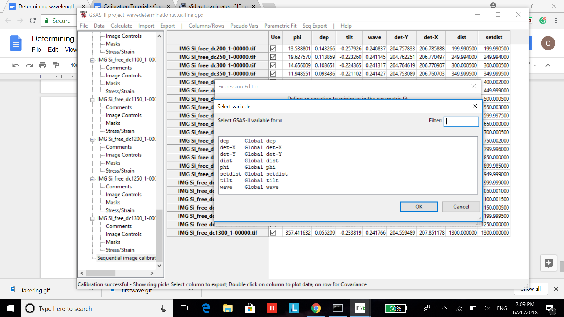
From the blank drop down bar select Global. A popup window will appear.

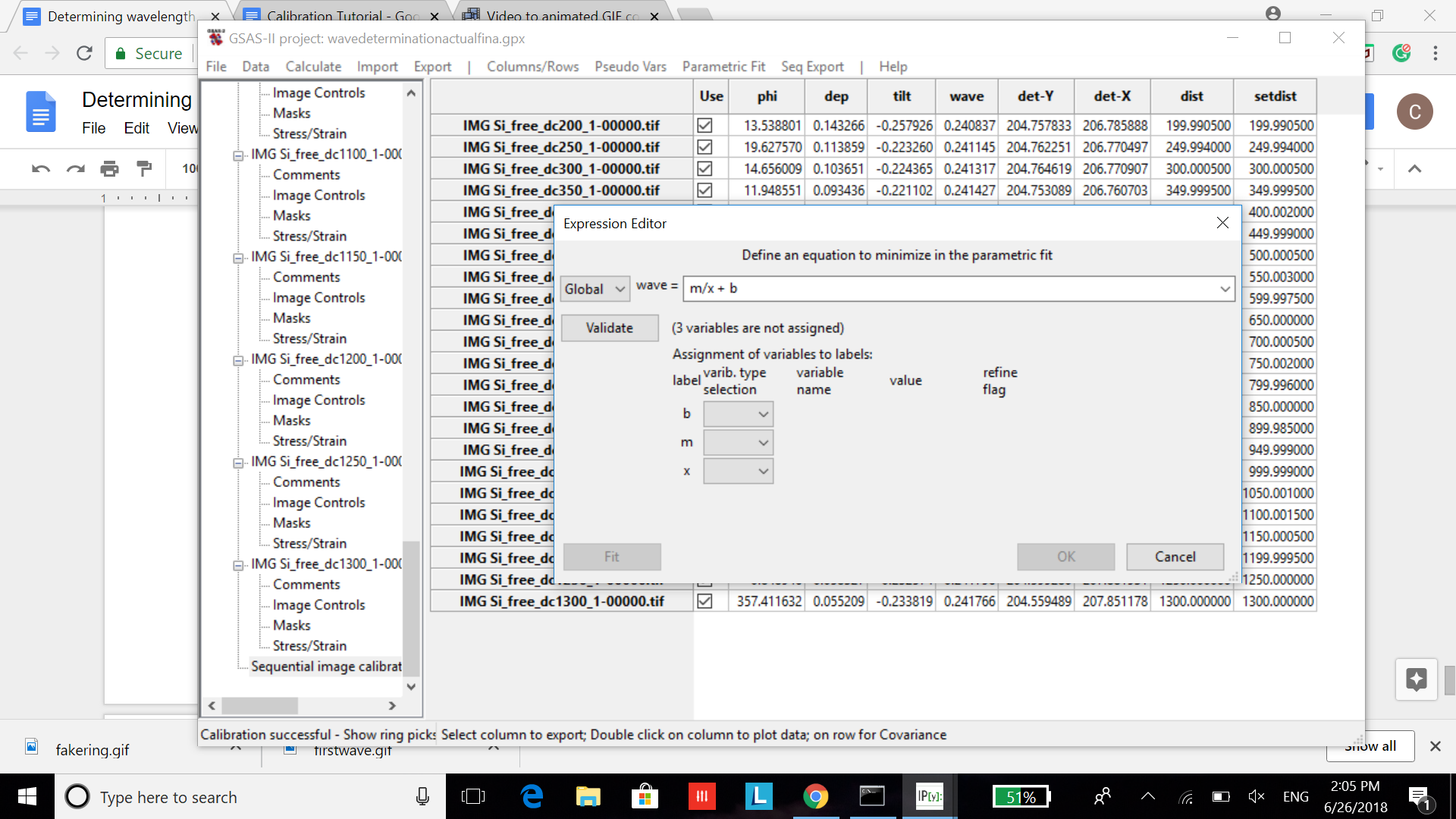
Select wave Global wave.  Then type in the equation: m/x + b and press Validate. The window will change and will allow you to enter variable types.

For both b and m variable type select Free. Then for x select Global.

Another popup window will appear.

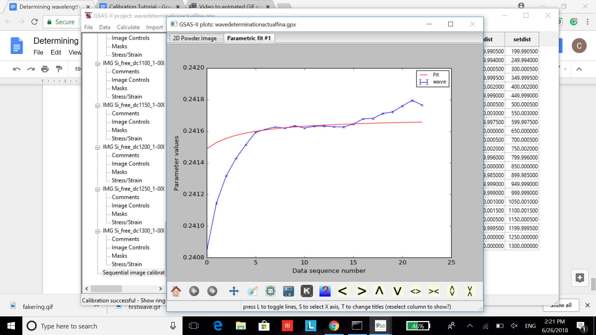
 Select setdist Global setdist. Then press Fit and observe the graph.

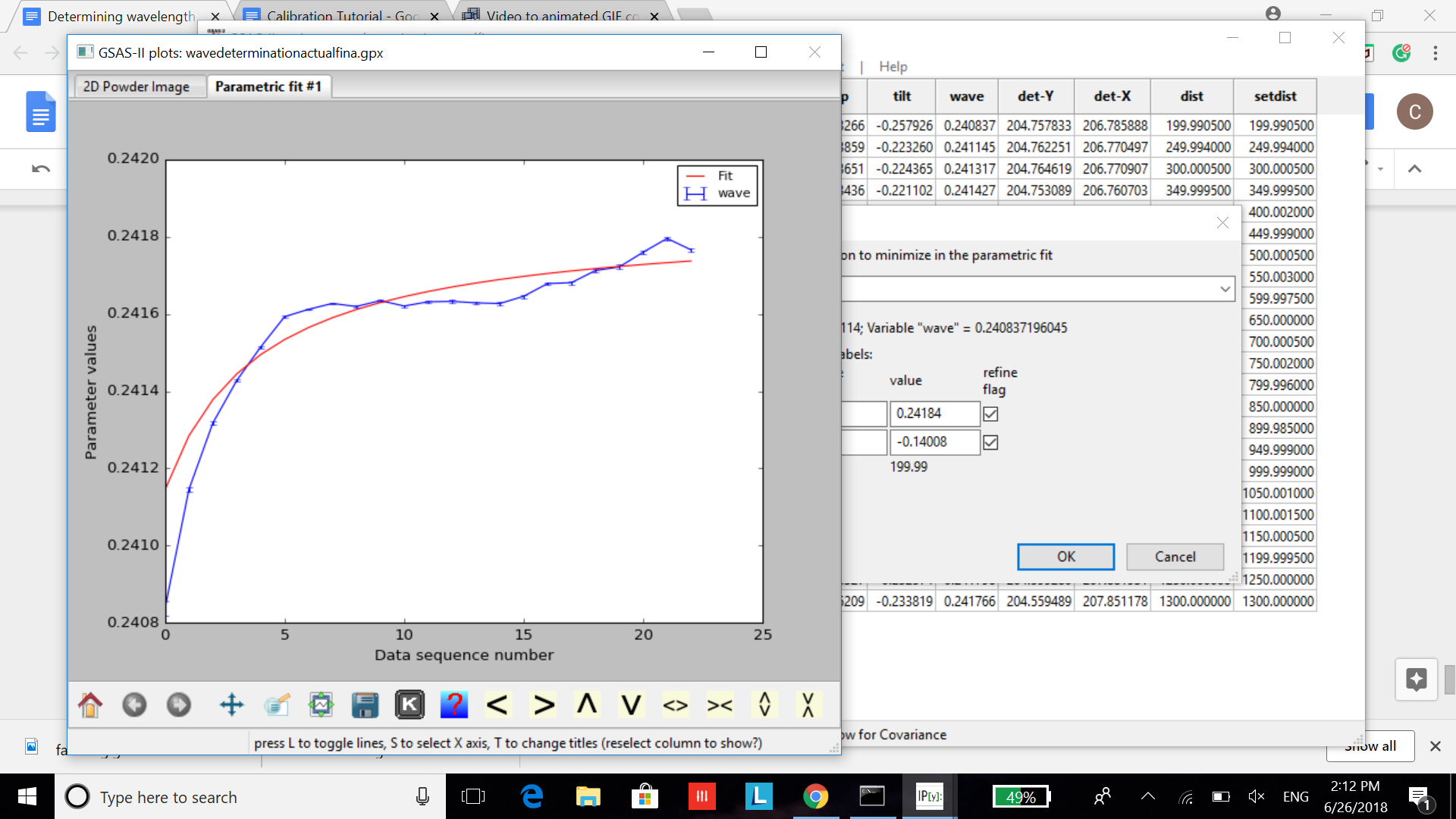
Note that the wavelength values vary significantly with dataset number (detector distance). This is a result of the detector distance being inaccurate. The fitting equation of "wave = m/dist + b" provides a first-order correction if the detectors are all offset by a particular amount. The fit looks reasonable, however, the images with detector placements that are very close are not as reliable since the offset has the largest impact and the ones very far away have very few rings and likewise should not be used. To make this change, we need to select OK so we are back to the table under Sequential image calibration results and deselect images so we only have a range from IMG Si_free_dc450_1-00000.tif to IMG Si_free_dc1000_1-00000.tif. The table should look like this:

Then select Parametric Fit/Edit Equation and then after the popup appears press Fit again. The new graph should show a much better fit.

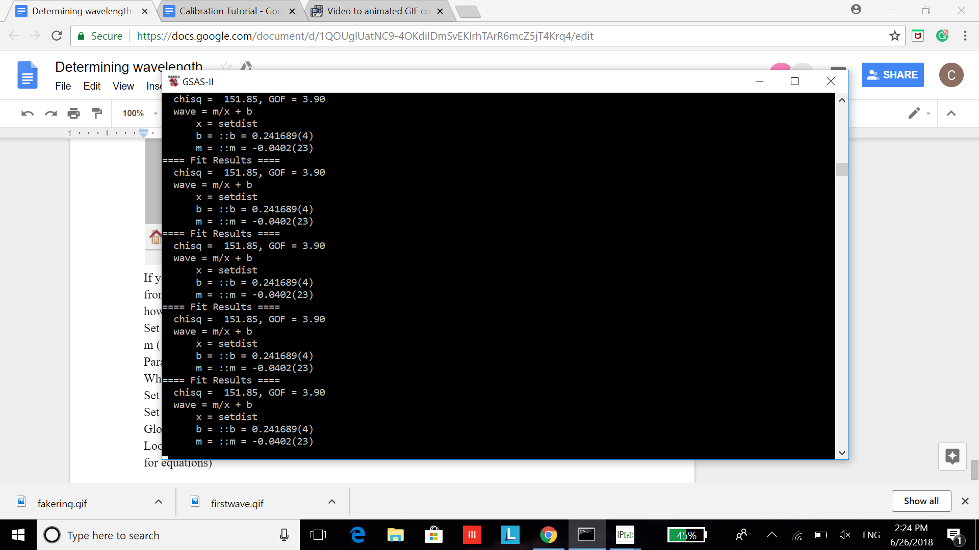
If you then go to the command prompt window, we know the variable b is the wavelength.

 So from this, we know that the average wavelength is 0.241689. Continue on to the next tutorial to learn how to use this calibration result to finish calibrating the distances.