Simulating Powder Diffraction with GSAS-II
While GSAS-II provides an environment
for fitting of diffraction data, it can also be used to simulate diffraction
experiments, where results are quantitative models for what can be expected,
provided that an accurate instrument description is used. Here we demonstrate
how a simulation is done for a two-phase mixture with multiple instrument
types.
Step 1: Read in Phases
First we will read in two phases, CuCr2O4
and CuO from files CuCr2O4.cif and CuO.cif, which can be downloaded from directory
https://advancedphotonsource.github.io/GSAS-II-tutorials/Simulation/data/.
Create a new project by starting GSAS-II
or by using the File/New Project menu item. Then use the Import/Phase/“from CIF
file” and select the CuCr2O4.cif for the “Choose Phase input file” dialog window.
Click “Ok” and “Yes” in the “Is this the file you
want?” confirmation window. The default
Phase name, CuCr2O4 is fine.
 Repeat this to read in the second phase: use the
Import/Phase/“from CIF file” and select the CuO.cif
for the “Choose Phase input file” dialog window. Click “Ok” and “Yes” in the “Is
this the file you want?” confirmation window. The default Phase name, CuO
is also fine.
Repeat this to read in the second phase: use the
Import/Phase/“from CIF file” and select the CuO.cif
for the “Choose Phase input file” dialog window. Click “Ok” and “Yes” in the “Is
this the file you want?” confirmation window. The default Phase name, CuO
is also fine.
Step 2: Create Simulation Histograms
Part A: Use the
Import/Powder Data/“Simulate a dataset” menu item (at bottom of menu list) to
create a simulation (dummy) histogram. The program then requests an instrument
parameter file name. Click Cancel and a list of default instrument parameters
are then displayed, as shown to the right. Select the APS 11-BM instrument
listing and press OK.
A dialog window is then displayed that with
the name for the histogram, the range of data and the step size. Below, note
that the name and start angle have been changed from the defaults. Then press
OK and the “Add to phase(s)” dialog is displayed.

Finally, in this dialog, we need to
indicate which phases are linked with this histogram. We want to include both
in the simulation, so use the “Set All” button (or select each phase) and press
OK.

Note that a new histogram is now added
to the data tree, as below. (Note the "Edit range" button which can be
used to change the values entered on the previous dialog).

Part B: Again use the
Import/Powder Data/“Simulate a dataset” menu item (at bottom of menu list) to
create a simulation (dummy) histogram. This time when the program then requests
an instrument parameter file name, supply file BT1.prm, which can also be
downloaded from directory
https://advancedphotonsource.github.io/GSAS-II-tutorials/Simulation/data/.

Click Open and a dialog opens for the
dataset name and range for this histogram. Change the range to 1 to 120 degrees
with 0.025 degree steps and optionally change the
name, as below.

Press OK and then the
“Add to phase(s)” dialog is displayed. As
before, add link both phases to this histogram. At this point a second histogram is shown in
the data tree:

Step 3: Set Scale Factor/Phase Fractions
 It is important to understand how the scale factor (found
each histogram's Sample Parameters tree entry) and phase fractions (found in
each phase's data tab) are used in GSAS-II. The scattering contribution for
each phase is set from the product of the histogram scale factor multiplied by
the phase fraction for each phase in that histogram which multiplies the
scattering power of each atom in the unit cell. This means that the phase
fraction effectively represents the relative number of unit cells present for
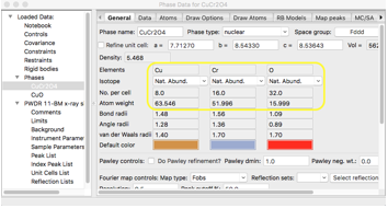
each phase. Note that after reading in the two phases in the previous step,
their phase fractions default to 1 for each. The contents of each phase are
shown on the General tab. Note that the unit cell contents for each phase are
Cu8Cr16O32 (1852.3 g/mol)
and Cu4O4 (318.2 g/mol), with
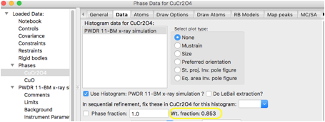
equal numbers of unit cells, the mass (or equivalently weight) fractions will
be 1852.3/(318.2+1852.3)=85.3% and 318.2/(318.2+1852.3)=14.7%. This can be
confirmed on the Data for each phase, as below.
It is important to understand how the scale factor (found
each histogram's Sample Parameters tree entry) and phase fractions (found in
each phase's data tab) are used in GSAS-II. The scattering contribution for
each phase is set from the product of the histogram scale factor multiplied by
the phase fraction for each phase in that histogram which multiplies the
scattering power of each atom in the unit cell. This means that the phase
fraction effectively represents the relative number of unit cells present for
each phase. Note that after reading in the two phases in the previous step,
their phase fractions default to 1 for each. The contents of each phase are
shown on the General tab. Note that the unit cell contents for each phase are
Cu8Cr16O32 (1852.3 g/mol)
and Cu4O4 (318.2 g/mol), with
equal numbers of unit cells, the mass (or equivalently weight) fractions will
be 1852.3/(318.2+1852.3)=85.3% and 318.2/(318.2+1852.3)=14.7%. This can be
confirmed on the Data for each phase, as below.
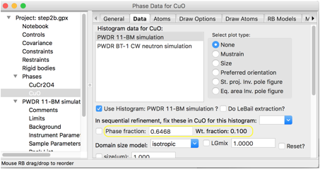
For this tutorial, we will choose to
set the mass fractions to give 90% CuCr2O4 and 10% CuO, so 90/1852.3=0.04859 and 10/318.2=0.03143. Equivalently,
we can normalize the phase fractions sum to 1 or so that either phase fraction is
1. We will use 1 for CuCr2O4, and 10*1852.3/(318.2*90)=0.6468
for CuO. Enter 0.6468 for the CuO
Phase fraction. When the mouse is moved
out of the box, the mass fraction to be recomputed and appears as 10%, as
expected:
This must be set for both histograms.
Clicking on the second histogram allows that phase fraction to be edited. Even easier
is to use the “Edit Phase”/“Copy data” menu item to copy all CuO data settings from histogram 1 to histogram 2. Note
that if the CuCr2O4 Data tab is selected for either phase,
the mass fraction is now shown as 90%.
Step 4: Turn off Optimization
A refinement computation is needed to
cause the pattern to be simulated. When a pattern is first simulated, the
observed pattern is set to the computed pattern (this can be reset by
using the "Edit range" button when the histogram data tree item is
selected. This means that it is actually
possible to optimize any parameters that are selected to be refined,
which can be used to test the sensitivity of different models refined
against a
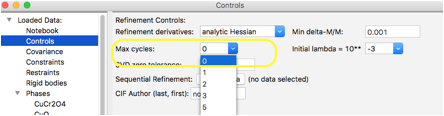
simulated dataset. In this case we only need to compute the simulated
pattern, so we will turn off optimization by setting the
number of cycles to zero. Do this by clicking on the Controls data tree entry and set the Max
cycles value to 0 using the pull-down menu:
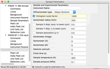
Step 5: Change Histogram Scale Factor
As discussed earlier, the range of intensities is determined by the histogram scale factor. For x-rays, a histogram scale factor with the default value of 1 produces a reasonable intensity range, but with CW neutrons, a much larger scale factor value is needed to produce a pattern with non-negligible intensity values. Note that GSAS-II adds simulated noise to patterns, so if the scale factor is too small, only random counts are seen. Select the Sample Parameters tree item for the second histogram and change the scale factor to 1000, as below.
Step 6: Simulate the Pattern
Use the Calculate/Refine menu item to
compute the simulated pattern. Clicking on the histogram entry in the data tree
causes the pattern to be displayed as below. This has the reflection tickmarks and the difference curve located at zero. While
both can be dragged to new positions, this is hard to do when they are obscured
by the “observed” and computed patterns. (The observed pattern has been set to
the computed pattern with the addition of simulated noise, which is why the
difference curve is non-zero.)

A nice trick for resetting the tickmarks to their usual default positions is to press “s”
to scale to sqrt(I) and press it again to return to normal scaling, as shown
below. These changes in scaling can also be done via the “K” (keyboard) button
on the bottom toolbar.

Note that the Commands menu offers menu
items for moving the difference curve and tickmarks,
as well as using drag and drop. Use of this, as well as using the rescaling graphics
toolbar item (the home button indicated by small house on the lower left)
allows more fine arrangement of locations. Exporting the plot (using the “floppy
disk” button allows the plots below to be created. Note the very big
differences in intensities, data range and resolution between the two
simulations.

