Simple Magnetic Structures in GSAS-II
Introduction
For magnetic neutron diffraction, the powder diffraction structure factor consists of two non-interacting components.
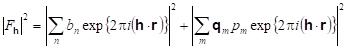
To have this result, one assumes that the neutron beam is not polarized and there is only elastic scattering. The first term is the ordinary nuclear structure factor found for all crystalline materials and the second is the magnetic scattering. Note that the result is a sum of squares implying that the nuclear and magnetic scattering intensities are summed to give the total that is measured in a magnetic powder diffraction experiment. This allows us to model the structure as two separate crystalline phases; one consists of the arrangement of all the atoms in the crystal structure described with a conventional unit cell and space group (the chemical or sometimes "nuclear" structure), and the other contains only the magnetic atoms in a perhaps different unit cell with a magnetic space group to describe the atom and magnetic moment arrangement (the magnetic structure). Needless to say the magnetic ions only have one set of positions, both phases must describe the same atomic arrangement; positions of the magnetic ions will be linked, as needed, by constraints between the phases in order to maintain this arrangement.
The magnetic scattering component has two factors

The second term (pm) is a scalar containing the magnetic form factor (fm), the magnetic moment magnitude (Sm) and a scaling factor ~0.539x10⁻¹² cm and is on the same scale as the normal neutron scattering lengths. Thus, magnetic scattering intensities are similar to those from the chemical structure. The first term (qm) depends on the projection of the magnetic moment onto the scattering vector for the reflection. If the scattering vector (unit vector εh) is parallel to the magnetic (unit vector Km) then the magnetic scattering intensity is zero and is large if the vectors are perpendicular. Thus, one can anticipate the direction of the magnetic moment in the structure by examining the observed magnetic intensities of low index reflections.
In this exercise you will use GSAS-II to determine the magnetic structure for a simple ferromagnet and a simple antiferromagnet. One is LaMnO3 which is an antiferromagnetic perovskite distorted by a strong Jahn-Teller distortion to an orthorhombic cell, and the other is LaMnO3 doped with enough Ca to make it a ferromagnet that is also orthorhombic. Neutron powder diffraction data for both were obtained on BT-1 at the NIST reactor at 50K (thanks to Qingzhen Huang for providing the data).
If you have not done so already, start GSAS-II.
Simple Antiferromagnet: LaMnO3
Step 1: Read in the data file
1. Use
the Import/Powder Data/from GSAS powder data file menu item
to read the data file into the current GSAS-II project. This read option is set
to read any of the powder data formats defined for GSAS (angles in centidegrees, TOF in µsec). Other submenu items will read
the cif
format or the xye
format (angles in degrees) used by Topas, etc. Because you used the Help/Download tutorial
menu entry to open this page and downloaded the exercise files (recommended),
then the SimpleMagnetic/data/... entry will bring you to the
location where the files have been downloaded. (It is also possible to download
them manually from https://advancedphotonsource.github.io/GSAS-II-tutorials/SimpleMagnetic/data/.
In this case you will need to navigate to the download location manually.)
For this tutorial you should see the data file in the file browser, but if
extensions on data files are not the expected ones, you may need to change the
file type to All files (*.*) to find
the desired file.
2. Select the LaMnO3_50K.gsas data file in the first dialog and press Open. There will be a Dialog box asking Is this the file you want? Press Yes button to proceed.
3. Since this data file does not define an instrument parameter file, a file dialog will appear for you to select the correct instrument parameter file. Select BT1_Cu300.inst; you may have to change the file type in the file selection Dialog box to GSAS iparm file to see it. At this point the GSAS-II data tree window will have several entries

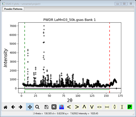
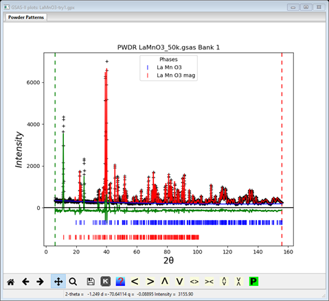
and the plot window will show the powder pattern

Step 2: Select Limits
This pattern has more data than we need, so it is helpful to cut down the range and one probably doesn’t want to use the two very broad peaks at the upper end of the pattern as they don’t contain much information for the magnetic structure. One also should be careful in selecting the lower limit especially for magnetic structure studies as a small peak may be hidden at low angles that can decisively determine a magnetic structure (there are none in this example, but this issue will be apparent in the next example). Click on the Limits item in the GSAS-II data tree. Use the New: set of entry boxes to set Tmin and Tmax to 6 and 156. Notice on the plot that the limit lines have moved to these positions; the green lower limit is just below the 1st peak and the red upper limit is just below that last two broad peaks. You may also drag the limit lines to the desired location or place them by a left mouse click on a data point for the lower limit or a right click on a data point for the upper limit. The plot should look like
Step 3: Read in the chemical structure for LaMnO3
1. Use the Import/Phase/from CIF file menu item to read the phase information for LaMnO3 into the current GSAS-II project. This read option is set to read Crystallographic Information Files (CIF). Other submenu items will read phase information in other formats. Because you used the Help/Download tutorial menu entry to open this page and downloaded the exercise files (recommended), then the SimpleMagnetic/data/... entry will bring you to the location where the files have been downloaded. (It is also possible to download them manually from https://advancedphotonsource.github.io/GSAS-II-tutorials/SimpleMagnetic/data/. In this case you will need to navigate to the download location manually.)
2. Select the LaMnO3.cif data file in the first dialog and press Open. There will be a Dialog box asking Is this the file you want? Press Yes button to proceed. You will get the opportunity to change the phase name next; press OK to continue.
3. Next is the histogram selection window; this connects the phase to the data so it can be used in subsequent calculations.
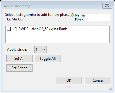
Select
the histogram (or press Set All)
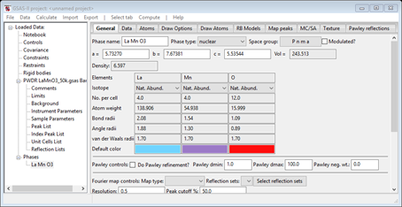
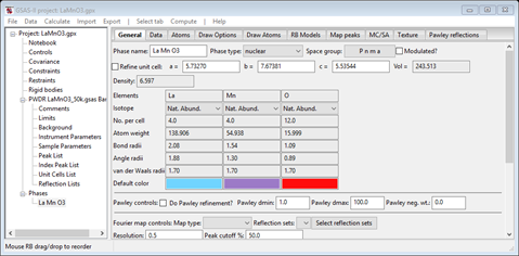
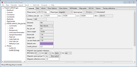
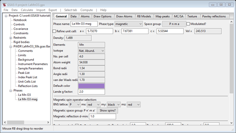
and press OK. The General tab for the phase is shown next
Step 4. Check powder pattern indexing
Here the objective is to determine how the reflection positions generated from the chemical (“nuclear”) crystal structure lattice match up with the peaks observed for this antiferromagnet.
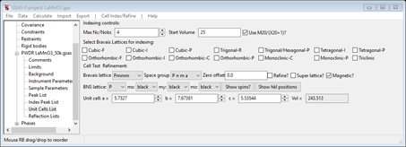
1. Select
Unit Cells List from the tree entries under the
histogram (begins with PWDR); the Indexing controls will be shown
This can use lattice parameters & space groups to generate expected reflection positions to check against the peaks in the powder pattern.
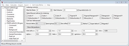
2. One
could then enter Bravais lattice, choose space group
& enter lattice parameters by hand, but the easy way is to use the chemical
lattice directly. Do Cell
Index/Refine/Load Cell from the menu; a Phase selection box will
appear with only one choice (LaMnO3).
This was taken from the Phases present in this project; there could be more
than one depending on what you loaded/created earlier. The Cell
Index/Refine/Import menu item allows you to get lattice information
from any one of the other phase containing files known to GSAS-II. Press OK and the Indexing controls will be change
showing the lattice constants for LaMnO3 you had obtained from the cif file. Note that the space group is set to that of the space
group for LaMnO3 (P n m a) and the lines will reflect the extinction
rules for this space group.
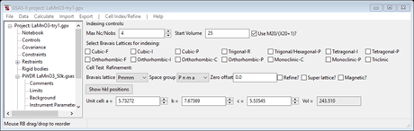
3. Change
the space group to P m m m to see all the
lines for this lattice (near the bottom of the pull down); the indexing will
immediately change

This is the reflection set for the Bravais lattice Pmmm which includes reflections that may be space group extinct and/or magnetically extinct. N.B., a reflection that is extinct due to the chemical structure space group could still be allowed for magnetic scattering.
4. Zoom
in on the lowest part of the pattern to see details of the indexing
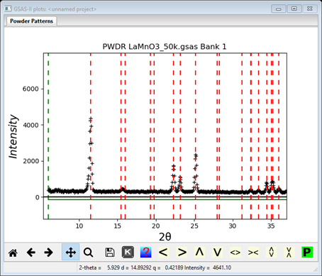
Note that every observed peak is indexed (unfortunately the peak at ~15.69°2Θ is probably a contaminant – it doesn’t exactly match the two calculated lines that straddle it).
5. Change the space group back to P m n a (near the bottom of the pull down); the indexing will immediately change
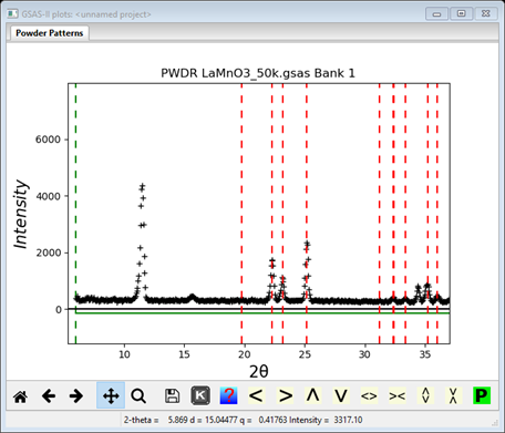
Notice that the 1st peak (as well as the contaminant) is no longer
indexed; this is likely to be a magnetic only peak as
expected from an antiferromagnet; there is another at ~34.4°2Θ. Reset the
space group to P m m m and put the cursor on these two in turn; a
popup box will tell you they are the (0,1,0) and (0,1,2) reflections. The two
straddling the contaminating peak are the (1,0,0) and
(0,0,1) reflections; they may be magnetically extinct. There are others that
show for Pmmm but vanish for Pnma
and have no visible intensity. We don’t know yet if they are magnetically
allowed or are zero because of the magnetic moment direction.
6. Reset the space group to P n m a; the reflections will again be updated. Then check the box Magnetic?; the tab will be changed showing some more options
and the powder indexing lines will also change showing every line to be indexed for the magnetic space group “P n m a”. However there are other spin selections (8 in all!) that might be possible. We have to introduce some “time reversal” operations (or “spin flips”). These are given by a choice of “red” or “black” for mx, my & mz (the 3 mirrors in Pnma). Try them out by selecting “black” or “red” for each; each time the plot will show the allowed reflections. Unfortunately this is not very definitive for selecting the magnetic space group; 4 choices will index the 1st line & 4 will not. The allowed ones are bbb, rrr, brb & rbr (b=black & r=red). In order to reject the rrr & bbb choices, you have to assume that the peak at ~15.69°2Θ is a contaminant and that the two reflections next to it 100 & 001 are indeed absent; this leaves two choices, Pn’ma’ and Pnm’a. If you press the ShowSpins? button, a popup window will appear showing the magnetic symmetry operators with spin inversion ones in red. For Pn’ma’ (e.g. rbr) the operators are
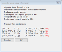
and the ones for Pnm’a (e.g. brb) are
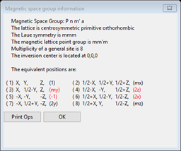
It is worthwhile noticing that the inversion operator (-1) is red in the latter but not in the former since an atom at an inversion center cannot have a magnetic moment if there is also spin inversion. More about this later. One other point is that certain space groups (e.g. P 212121) only allow an even number of spin inversions; GSAS-II will always enforce this by setting the spin flags accordingly, so getting a desired arrangement might take a bit of trial-and-error selection to get what you want. Press OK to get rid of the popup box. To narrow down the choice we have to examine what happens to the atoms for each choice. In some cases the choice might not allow the Mn atom to have a magnetic moment so it must be rejected. We will try this in the next step.
Step 5. Make the magnetic phase
In the previous step we did not have to resort to any doubling of a cell axis to explain the suite of magnetic reflections, so the propagation vector is zero (we will see this in later magnetic tutorials). To make the magnetic cell from the chemical cell we will use the transform tool that is in GSAS-II in the General tab for the chemical structure. That tab is
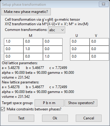
Under the Compute menu item do Transform; a new popup dialog box will appear with stuff needed to effect a cell transformation.
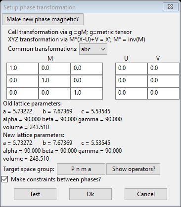
The order of operations for the transformation is given at the top of the window; the U vector permits applying an origin shift to the atom coordinates before the transformation and the V vector is for an origin shift after the transformation. The lattice parameters are transformed by changing the metric tensor via
g’ = gM
The atoms positions are transformed via
X’ = M*(X-U)+V
where M* is the inverse of the transformation matrix. The anisotropic thermal parameters are transformed via
U’ = MTUM/det(M)
The dialog box gives an extensive list of commonly used transformations for e.g. swapping axes. In this case we are not transforming the unit cell so the matrix is just the unit matrix (ones on diagonal) and we are not shifting the origin so U & V are zeros. We do want the new phase to be magnetic so press the Make new phase magnetic button; the dialog will be redrawn
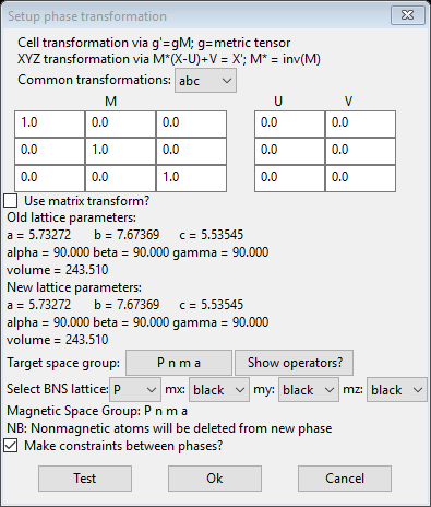
This allows one to select possible magnetic spin inversions and lattice centering operations as given by the BNS nomenclature. This can be needed if one had discovered a requirement of doubling a cell axis in the previous step (e.g. a nonzero propagation vector). This is not required in this case and we are using the space group (Pnma) for the magnetic cell; we will be setting the spins (mx,my,mz) later as well. Leave the box at the bottom about constraints checked as we want them to tie the two phases together. Press Ok to continue; a new popup will appear
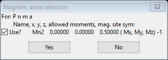
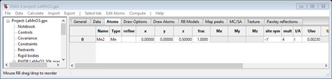
You see the magnetic atom position, allowed magntic moments and magnetic site symmetry.
This allows one to reject certain atoms that are known to not be magnetic; press Yes to continue. A new phase will be created and the General tab for it will be shown.

The phase is named with “mag” appended to the end, the phase type is magnetic and there are magnetic spin operator selections part way down the page. You also can see the Lande’ g factor can be changed if needed and it only contains the Mn atom. To see what happened with respect to constraints, select Constraints from the main part of the GSAS-II data tree. The ones for phases will be shown
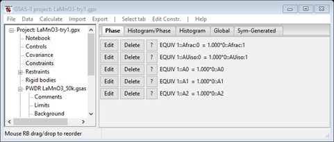
This shows all the possible required constraints between the chemical structure and the magnetic one (the ones for Uij are not generated). The first two are for the Mn atom; only the Uiso one is probably necessary for this analysis but the other one will do no harm. The last three tie the lattices together. Select the Histgram/Phase tab

This gives the constraints between the two phases for scale factors (e.g. phase fractions) and the size & mustrain sample broadening terms. NB: this assumes isotropic modelling of both because the original LaMnO3 was modeled that way. If you want to use one of the more complex sample broadening models, you will have to revisit this tab and put in the appropriate entries to tie those parameters together.
Step 6. Select spin configuration
Recall that we had found 2 spin configurations that were consistent with the observed peaks; Pn’ma’ and Pnm’a (there was also the possibility of Pnma or Pn’m’a’ if one chose not to ignore that contaminating peak at ~15.69°2Θ). First let’s try Pnm’a; select “red” for the middle spin selector (my); the window will be refreshed. Then select the Atoms tab; it will show
The boxes that carry the magnetic moment components (Mx, My & Mz) are grey indicating that no magnetic moment is allowed for the Mn atom site in the space group Pnm’a. The site symmetry is marked as -1’ indicating an inversion center with spin inversion; this precludes a magnetic moment. So we need to try the other choice, Pn’ma’. Return to the General tab and change the mx, my & mz spin operators to “red”, “black” & “red”, respectively. The tab will refresh at each change. When done it should look like
It now shows the magnetic space group as Pn’ma’. The Atoms tab now shows

with 0.0 in each of the magnetic moment components, because the site symmetry is -1 which allows a magnetic moment. We can now give the Mn atom a magnetic moment. You can also try the other two choices, Pnma and Pn’m’a’. The latter can be rejected immediately because the -1 operator has spin inversion (use the Show spins? button to show the operators), leaving only Pnma as a possibility along with Pn’ma’. Both allow the Mn site to have a magnetic moment. Put the choice to Pn’ma’ (“red”, “black” & “red”); we’ll test Pnma later. This might be a good place to save the project; I called it “LaMnO3.gpx”.
Step 7. Solving the magnetic structure
1. Test the Pn’ma’ model
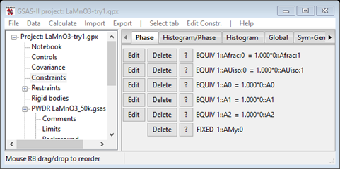
So now we have one or maybe two spin arrangements to consider, Pn’ma’ and possibly Pnma, but we do not know the magnetic moment components, Mx, My & Mz. However, since the 1st reflection (the 010) is magnetic and strong, it is likely that the value of My=0. We can force this (to avoid refinement problems) by making a ‘hold’ on its value. Select the Constraints item from the GSAS-II tree; it will show the constraints generated when the magnetic phase was made

Under the Edit Costr. menu item do Add hold; a Hold phase variable window will appear
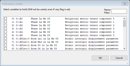
Scroll down to the bottom and select 1::AMy:0 and press OK. The constraints will have a new entry giving the hold on My for the Mn atom at the bottom of the list.
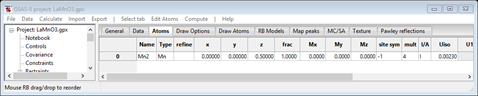
Now return to phases and select La Mn O3 mag and the Atoms tab; you should see

The least squares will not begin a refinement of Mx & Mz starting from zero since either +/- values are equally possible; the result will be a singularity. So these values must be offset so set them to 1.0 each. Save the project as LaMnO3 try1. Do Calculate/Refine; the refinement will quickly converge to Rwp ~14% and the powder plot will look like
There does not appear to be any calculated magnetic intensity, but a zoom onto the low angle (10-30°2Θ) part of the pattern shows that some intensity was obtained, but clearly not enough.

The magnetic moment is clearly too small; to let the least squares find a better value set the refine flag for Mn to ‘M’ and repeat Calculate/Refine. The residual will drop considerably to Rwp ~8.7% and the low angle portion will show a much better fit.
This appears to be a reasonable solution; a more complete refinement still needs to be done, we’ll do that in the next step after we test the Pnma model. Save the project (should be LaMnO3 try1).
2. Test the Pnma model
Now reopen the original LaMnO3.gpx file saved at the end of Step 6 above. Select La Mn O3 mag phase from the GSAS-II tree; the General tab will be shown
Now set the spin operators to all “black” for Pnma and then select the Atoms tab
Again, one can make the same argument that since the 010 reflection is large then My should be zero. Set Mx & Mz to 1.0 and then go to Constraints and set the hold on 1::AMy:0. Save the project as LaMnO3 try2. Do Calculate/Refine from the main menu to do a Rietveld refinement. It converges to Rwp ~14%; about the same as the Pn’ma’ model at the same step. The low angle portion of the powder pattern shows

There is intensity in the lowest angle reflection (the 010) but not enough. Again we’ll try to refine the Mx & Mz components to see what happens. Set the refine flag for Mn to ‘M’ and repeat Calculate/Refine. The residual will drop to Rwp ~10% and the low angle portion will show a much better fit which is very similar, but slightly poorer than the result from the Pn’ma’ model. To see how, examine a slightly higher angle region (30-55°2Θ) and compare it with the same region for the plot for the Pn’ma’ model (you’ll need 2 instances of GSAS-II running to do this)


You can see in particular at the pair of peaks at 33.3 and 34.4°2Θ that are well fit by the Pn’ma’ model and not by the Pnma one. On this basis the Pnma model is rejected and the Pn’ma’ is selected as probably correct. NB: neither model produced any intensity for the peak at ~15.69°2Θ, so it is most likely to be from a minor contaminating phase; we can either ignore it or exclude it in the final refinements.
Step 8. Complete refinement of the Pn’ma’ model for LaMnO3
Reload the LaMnO3 try1.gpx project file which should have the Pn’ma’ model for the magnetic structure, and look at the powder pattern to decide how to proceed to complete the refinement.

Looking at the plot, it would seem that the lattice parameters and sample position need to be refined. It is important to remember that if a parameter in one phase is varied then the corresponding one in the other phase must also be varied, otherwise GSAS-II will report the error and refuse to attempt the refinement. To set refinement of the lattice parameters, bring up the General tab for each phase & check the Refine unit cell box for the lattice parameters. Then select Sample Parameters for the PWDR entry
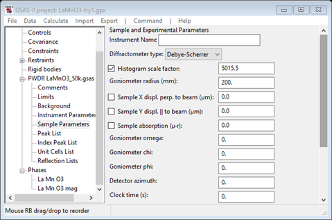
Since the scan covers a very wide range in 2Q, both sample displacements can be refined. Check both Sample X and Y displ parameters. NB: if the correct Goniometer radius (650mm) is used, these displacements will be in microns. Also, it would appear that the instrument parameters do not adequately describe the anisotropic broadening of the lowest angle reflection so we will need to include that. Select Instrument Parameters from the PWDR entry and check the SH/L Refine box. Now do Calculate/Refine until convergence is achieved (i.e. Rwp doesn’t change). This will be 2-3 times. When done my Rwp was ~6.6% with a nice clean plot

Now we can add refinement of the atom positions and thermal parameters. For Atoms tab of the La Mn O3 phase, double click the refine column heading and select X & U. This will add these parameters as allowed by symmetry to the refinement. Now go to the Atoms tab for La Mn O3 mag and double click the refine tab. Select U & M; the Uiso for the Mn atom is tied via a constraint to the Mn in the other phase. Now select Background from the PWDR entry and increase the number of terms to 6. Finally do Calculate/Refine until convergence (1-2 times). My Rwp was 6.29% with a plot that is hardly different from the previous one. If you press the ‘W’ key with the focus on the plot, GSAS-II will show the weighted difference curve below the plot

This curve shows a couple of peaks which are from some contaminating phase, but otherwise the fluctuations are mostly within 2s of zero. Finally examine the magnetic moment components of the Mn atom; Mz is close to zero. It is likely that it is zero; set it to zero and then go to the Constraints tree item and add a hold for the 1::AMz:0 parameter so that it stays at zero. Repeat the refinement; the residual is unchanged showing that setting Mz=0 was a valid assumption.
Step 9. Draw the magnetic structure of LaMnO3
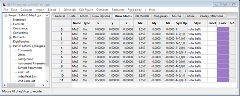
To draw the magnetic structure select the Draw Atoms tab for the magnetic phase. The table will have a single line matching that of the Atoms table with a few extra columns.

The plot will show one atom with magnetic moment. Select the atom in the table and do Edit Figure/Fill unit cell. The table will show additional entries
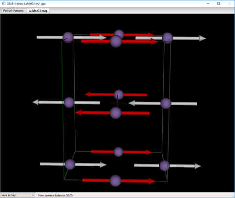
The plot will show the unit cell contents of Mn atoms each with its magnetic moment; they are arranged in layers along the b-axis with the moments antiparallel from one layer to the next. Some are red indicating that a spin inversion operation was applied for that atom moment.
This completes this tutorial; you can save the project if you wish & close GSAS-II.
Simple Ferromagnet: La0.7Ca0.3MnO3.
The magnetic structure of LaMnO3 can be profoundly changed by addition of Ca in place of some of the La; in this case ferromagnetic ordering apparently was obtained. This tutorial will investigate that from neutron powder data collected at 50K on the same instrument as the first exercise (BT1 at NIST; thanks to Qingzhen Huang for providing the data). Start GSAS-II if you have not done so already.
Step 1: Read in the data file
1. Use
the Import/Powder Data/from GSAS powder data file menu item
to read the data file into the current GSAS-II project. This read option is set
to read any of the powder data formats defined for GSAS (angles in centidegrees, TOF in µsec). Other submenu items will read
the cif
format or the xye
format (angles in degrees) used by Topas, etc. Because you used the Help/Download tutorial
menu entry to open this page and downloaded the exercise files (recommended),
then the SimpleMagnetic/data/... entry will bring you to the
location where the files have been downloaded. (It is also possible to download
them manually from https://advancedphotonsource.github.io/GSAS-II-tutorials/SimpleMagnetic/data/.
In this case you will need to navigate to the download location manually.)
For this tutorial you should see the data file in the file browser, but if
extensions on data files are not the expected ones, you may need to change the
file type to All files (*.*) to find
the desired file.
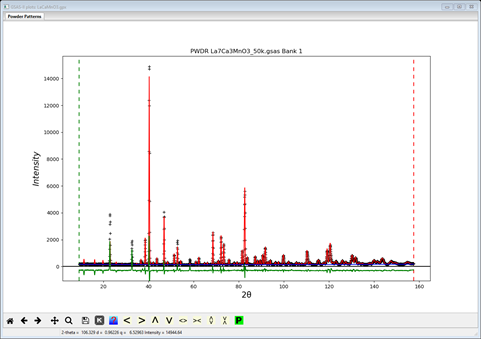
2. Select the La7Ca3MnO3_50K.gsas data file in the first dialog and press Open. There will be a Dialog box asking Is this the file you want? Press Yes button to proceed.
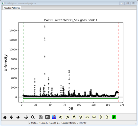
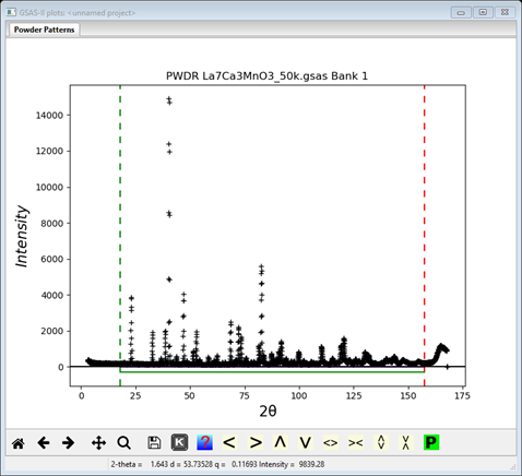
3. Since this data file does not define an instrument parameter file, a file dialog will appear for you to select the correct instrument parameter file. Select BT1_Cu300.inst; you may have to change the file type in the file selection Dialog box to GSAS iparm file to see it. At this point the GSAS-II data tree window will have several entries

and the plot window will show the powder pattern
Step 2: Select Limits
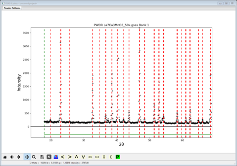
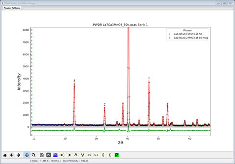
This pattern has more data than we need, so it is helpful to cut down the range. Click on the Limits item in the GSAS-II data tree. Use the New: row of entry boxes to set Tmin and Tmax to 18 and 157.5. Notice on the plot that the limit lines have moved to these positions; the green lower limit is just below the small 1st peak (at ~20°2Θ) and the red upper limit is just below that last broad hump. You may also drag the limit lines to the desired location or place them by a left mouse click on a data point for the lower limit or a right click on a data point for the upper limit.
Step 3: Read in the chemical structure for La0.7Ca0.3MnO3
1. Use the Import/Phase/from CIF file menu item to read the phase information for LaMnO3 into the current GSAS-II project. This read option is set to read Crystallographic Information Files (CIF). Other submenu items will read phase information in other formats. Because you used the Help/Download tutorial menu entry to open this page and downloaded the exercise files (recommended), then the SimpleMagnetic/data/... entry will bring you to the location where the files have been downloaded. (It is also possible to download them manually from https://advancedphotonsource.github.io/GSAS-II-tutorials/SimpleMagnetic/data/. In this case you will need to navigate to the download location manually.)
2. Select the LaCaMnO3.cif data file in the first dialog and press Open. There will be a Dialog box asking Is this the file you want? Press Yes button to proceed. You will get the opportunity to change the phase name next; press OK to continue.
Next is the histogram selection window; this connects the phase to the data so it can be used in subsequent

Select the histogram (or press Set All) and press OK.
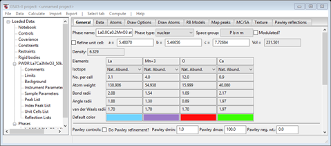
The General tab for the phase is shown next
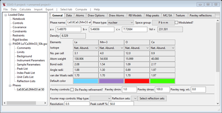
Notice that the space group from the cif file is Pbnm; this is a nonstandard setting of Pnma. GSAS-II can treat this case just as well as the standard setting so we can proceed without any concern.
Step 4. Check powder pattern indexing
Here the objective is to determine how the reflection positions generated from the chemical (“nuclear”) crystal structure lattice match up with the peaks observed for this antiferromagnet.
Select Unit Cells
List from the tree entries under the histogram (begins with PWDR);
the Indexing controls will be shown
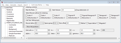
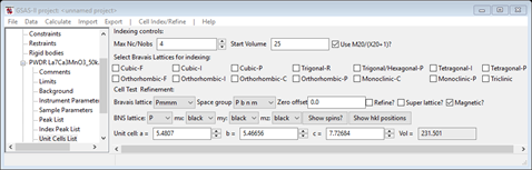
This can be use lattice parameters & space groups to generate expected reflection positions to check against the peaks in the powder pattern. Do Cell Index/Refine/Load Cell from the menu; a Phase selection box will appear with only one choice. This was taken from the Phases present in this project; there could be more than one depending on what you loaded/created earlier. The Import menu item allows you to get lattice information from any one of the other phase containing files known to GSAS-II. Press OK and the Indexing controls will be change
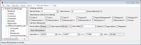
showing the lattice constants and space group (P b n m) for LaCaMnO3 you had obtained from the cif file.
Change
the space group to P m m m; after a short
pause (while reflections are generated), the plot will show the calculated
reflection line positions. Zoom in on the lowest part of the pattern to see
details of the indexing 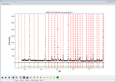
Note that almost every observed peak is indexed; even the two weak peaks that are on either side of the 1st strong peak. More about those later. There is also a few seemingly misplaced unindexed lines (at 37.4, 53.9 & 67.4°2Θ); probably some contaminating minor phase. We’ll have to ignore them. Change the space group back to P b n m; the indexing will change.
Then check the box Magnetic?;
the tab will be changed showing some more options
Because the sample is ferromagnetic, all the magnetic scattering could be expected to coincide with the scattering from the chemical cell. There are no extra reflections; making it difficult to discern which spin configuration is appropriate without knowing the scattering from the chemical cell. Changing the spins will cause the lowest index lines to be extinct (as antiferromagnetic selections are made); these can be seen by moving the lower limit to below 10°2Θ. The problem is that they may have no intensity because of the moment directions, e.g. if only Mx ≠ 0, then all Fh00 (parallel to the moment) will be zero even if allowed by the magnetic symmetry. Thus, we will have to defer this testing until after we have a computed pattern from the chemical cell and can compute some trial patterns from the magnetic cell.
Step 5. Make the magnetic phase
In the previous step we did not have to resort to any doubling of a cell axis to explain the suite of magnetic reflections, so the propagation vector is zero. To make the magnetic cell from the chemical cell we will use the transform tool that is in GSAS-II in the General tab for the chemical structure. That tab is
Under the Compute menu item do Transform; a new popup dialog box will appear with stuff needed to effect a cell transformation.
The order of operations for the transformation is given at the top of the window; this was described in the 1st part of this tutorial. We do want the new phase to be magnetic so press the Make new phase magnetic button; the dialog will be redrawn
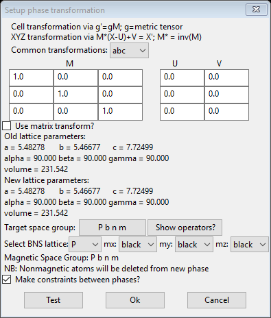
This allows one to select possible magnetic lattice centering operations as given by the BNS nomenclature and the spin inversions mx, my & mz (we will do these later). This can be needed if one had discovered a requirement of doubling a cell axis in the previous step (e.g. a nonzero propagation vector). This is not required in this case and we are using the same nonstandard space group (P b n m) for the magnetic cell that is used for the chemical cell. Leave the box at the bottom about constraints checked as we want them to tie the two phases together. Press Ok to continue; a new popup will appear

This allows one to reject certain atoms that are known to not be magnetic; press Ok to continue. A new phase will be created and the General tab for it will be shown.
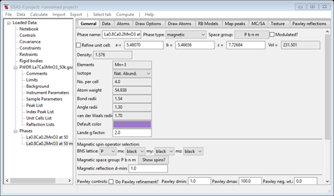
The phase is named with “mag” appended to the end, the phase type is magnetic and there are magnetic spin operator selections part way down the page; they are all “black”. You also can see the Lande’ g factor can be changed if needed and the phase only contains the Mn atom. As before the appropriate constraints have been built linking the two phases together. Look at Constraints if you wish to see them.
Step 6. Select spin configuration
Select the Atoms tab, the parameters for Mn are shown
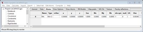
Notice that Mx, My & Mz are shown with 0.0 for each and the site symmetry is “-1”; an inversion with no spin flip allows the site to have a magnetic moment. So the all “black” configuration is possible on the basis of the Mn site symmetry. If you make one of the spin operators “red” (say mx) and then press Show spins?, the popup will show a red (-1) symbol indicating that the inversion operation (#5) also has a spin inversion. This spin arrangement wouldn’t allow the Mn to have a moment so it must be rejected.

The Atoms tab would show Mx, My & Mz as gray indicating that they cannot have a nonzero value.

If you try other spin configurations this way, you will quickly see that an odd number of spin flips will yield for Pbnm inversions centers with spin flips and all must be rejected on that basis leaving only configurations with an even number of spin flips (e.g. “bbb”, “rrb”, “rbr” and “brr”) for which the inversion center does not have a spin flip and thus can carry a magnetic moment. We will have to test each in turn, moreover the moment direction also needs to be established (e.g. values of Mx, My & Mz).
Step 7. Solving the magnetic structure - Trial and Error
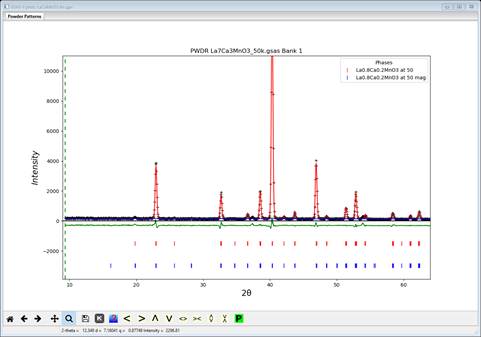
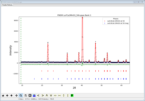
Because of the equivalence of ± Mx, ± My and ± Mz, the least squares will show singular matrix behavior if any are started at zero. So we must begin any test refinement with nonzero moment components. We may discover later that some moment component is nearly zero; it can then be set to zero and a hold placed on that value to avoid the singularity. We will need to test each spin configuration in turn & then compare them to find the best one. To proceed select the the magnetic phase and set the spins to “bbb” (i.e. all “black”). Then select the Atoms tab and enter 1.0 for each of Mx, My & Mz; this provides a suitable starting point. The default refinement is just scale factor & background; do Calculate/Refine. It will quickly converge to Rwp ~15.5% and the plot will look like
Clearly there is intensity mismatches at low angles because the magnetic structure is incorrect, but there is also misfits due to peak position errors. We can refine lattice parameters and sample position to address this. Select each phase in turn and select Refine unit cell on the General tab for each; the constraints connecting them were built earlier by the Transform operation in GSAS-II. Next select Sample Parameters under the PWDR entry and select Sample X displ and Sample Y displ for refinement; change Goniometer radius to 650 so the result is in microns. Now do Calculate/Refine again; Rwp will drop slightly (mine was ~13.6%). Save the project, and do a Save Project as.. and name it LaCaMnO3 bbb.gpx (the gpx is assumed & the ‘bbb’ refers to the all black configuration which we will test next. The saved LaCaMnO3.gpx will then be our starting point for testing the spin configurations.
1. Test the bbb configuration – Pbnm
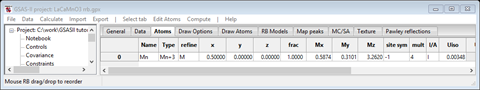
To test the magnetic configuration, we need to refine the magnetic moment components to obtain the optimal values for the spin configuration and thus the best fit. Select the magnetic phase and go to the Atoms tab. Then double click the refine column heading and select ‘M’ from the popup dialog. It should look like

Then do Calculate/Refine from the main menu, it converges quickly (Rwp ~11.8%) and still a poor fit for the low angle reflections

and the magnetic moment components are

So we test the next possibility.
2. Test the rrb configuration – Pb’n’m
Since we want to be able to compare results, start a new GSAS-II and open the LaCaMnO3.gpx project. Immediately do a Save Project as… and name it LaCaMnO3 rrb.gpx (this step might easily be forgotten and then your reference starting structure will be lost!). Then select the magnetic phase and the General tab is displayed. Set the spin configuration to “red”, “red” & ”black”. Then go to the Atoms tab and set the refine flag to ‘M’; then do Calculate/Refine. The residual will immediately drop to Rwp ~8.0% which is much better than the “bbb” spin configuration and the plot gives a far better fit to the low angle peaks
The Atoms tab shows a very strong Mz component ot the magnetic moment on Mn with the other two components near zero.
Let’s test the next one.
3. Test the rbr configuration – Pb’nm’
Again start a new GSAS-II with the reference project LaCaMnO3.gpx and immediately Save project as.. with the name LaCaMnO3 rbr.gpx. Then select the magnetic phase and the General tab is displayed. Set the spin configuration to “red”, “black” & ”red”. Then go to the Atoms tab and set the refine flag to ‘M’; then do Calculate/Refine. The residual will be just a bit poorer (Rwp ~8.2%) than the “rrb” model. The plot is very similar
The Atoms display shows a strong My moment component with Mx & Mz small

We should now check the last spin configuration.
4. Test the brr configuration – Pbn’m’
As before, start a new GSAS-II with the reference project LaCaMnO3.gpx and immediately Save project as.. with the name LaCaMnO3 brr.gpx. Then select the magnetic phase and the General tab is displayed. Set the spin configuration to “black”, “red” & ”red”. Then go to the Atoms tab and set the refine flag to ‘M’; then do Calculate/Refine. The residual virtually the same as the “rrb” model (Rwp~8.0%) but better than the “rbr” one. The plot is very similar
and with the strong Mx moment component with My & Mz small.
Clearly the “bbb” configuration is not correct, but which one of the other three is difficult to choose at present. Let’s complete the refinement on each one and see where that leads. All that is required is to add the remaining atom parameters (X & U). For each of the “rrb”, “rbr” and “brr” models go to each phase Atoms tab and change the refinement flags to XU for the chemical ones and UM for the magnetic ones. Also make the number of Background terms 6 for each; that will provide slight improvement as well. The do Calculate/Refine for each one. After several cycles of refinement I find the “rrb” model Rwp=7.615%, the “rbr” model Rwp=7.716% and the “brr” model Rwp=7.591%.
Finally, if one examines the Atom tabs for the “rrb” and “brr’ models, the My component of the magnetic moment is quite close to zero (My ~0.2) for both. Set it to zero in both cases and add the hold on 1::AMy:0 in the Constraints for each as well to keep them at zero. Repeat Calculate/Refine. I got Rwp=7.616% for the “rrb” model and Rwp=7.558% for the “brr” model indicating a slight preference for the latter. A very close look at the peak at 32.7°2Θ gives some indication of where this small difference in residual comes from (“rrb” on left & “brr” on right).The plots are the square root of intensity and the weighted difference is shown below.


The magnetic peaks contributing to this peak are the 200,221 & 020 for the “rrb” model; for the “brr” model the 200 is absent. This extra reflection makes a contribution to the profile for “rrb” that makes the fit slightly worse than for the “brr” model. Thus, the correct magnetic structure can be assigned for La0.7Ca0.3MnO3 as Pbn’m’ (not Pb’n’m). The structure looks like
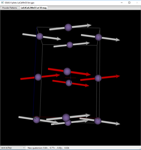
which shows that the ferromagnetic arrangement is slightly canted in the z-direction (Mz =0.50) with the major component (Mx =3.25) along the x-axis. A test refinement with Mz = 0 gives a slightly poorer fit Rwp=7.596% vs 7.591% and fails to put any calculated intensity into the 1st weak peak (101 & 011) at 19.82°2Θ thus confirming that the canting is apparently real.
This completes the “simple magnetic structure” tutorials.