Sequential refinement of multiple datasets –
CuCr2O4 from 7K to 300K
Sequential refinement is a way to fit a series of datasets collected under similar conditions with a set of closely related models. Each dataset receives an independent fit. Thus it is possible to track how the models evolve over the course of the measurements. One or more phases may be used to fit all all the datasets or some phases may appear in just some of the measurements, should there be phase transitions.
Sequential refinements can be performed in three different ways:- where the resulting parameters after a fit for a histogram are used as the starting point for the next histogram.
- with differing starting parameters for each histogram
- with the same starting parameters for each histogram
In this example, we will fit a temperature series where both the unit cell and atomic parameters evolve with temperature. Note that it is also possible to fit a temperature series as a combined refinement and, as will be seen, one can still deal with thermal expansion (using the Hydrostatic/Elastic strain terms), but a combined refinement would allow only a single set of (averaged) atomic parameters for all temperatures. A sequential refinement allows each data set to determine the atomic parameters and allows their variation with temperature to be determined.
Data for this example will be downloaded with the tutorial, if you used that option to see this page. Otherwise, download file SeqTut.zip from here. This example assumes that one is already familiar with use of GSAS-II for simple refinements. Note that menu entries are listed in bold face below, such as Help/About GSAS-II, which lists first the name of the menu (here Help) and second the name of the entry in the menu (here About GSAS-II).Step I: Fit a single temperature.
If you have not done so already, start GSAS-II. While it is possible to start a sequential refinement reading in all phases and datasets from the beginning, usually it is best to know something about how the fit will be performed and this usually means performing one or more fits to representative individual datasets as the conditions or phases present change. One way to do this could be to read in all datasets but select only a single individual dataset for that fit until we are ready to fit the entire sequence. Here we will start by reading in only the first dataset and fit that. Then we will add more datasets and perform a sequential fit.1. Read phase files CuCr2O4.cif and CuO.cif from file SeqTut.zip.
- Use the Import/Phase/from CIF file menu item to read the phase information. In the file browser dialog window that is created, change the file type from “CIF file” to “zip archive” and select the SeqTut.zip file (change the file directory to SeqRefine/data). Another dialog window will be created showing all the files in the zip archive. To simplify the view to only show the phase files, type “cif” (or “CIF” – case is ignored) into the filter. Select the CuCr2O4.cif and the CuO.cif input files. Press OK. (If this exercise is being repeated, files CuCr2O4.cif or the CuO.cif will already exist. If so, you will be asked to OK overwriting them.)
- You will be asked sequentially for the name for each phase. The defaults (CuCr2O4 and CuO) are fine, so OK can be pressed for each question.
- Note that for CuCr2O4, the space group (Fddd) can
be set with two origin choices. Select Keep current coordinates
since the coordinates are already set properly.
Discussion:
When there is a choice, GSAS-II requires the use of Origin 2, which
places the origin at a center of symmetry, and this CIF has been set
that way
(the presence of a -x,-y,-z symmetry operation confirms that), but GSAS-II
notes the possible choice and offers to apply the shift to the
coordinates that would shift from Origin 1 to Origin 2.
As shown in the window where this
choice would be made, this shift were applied,
the unit cell contents would be
Cu16Cr8O32 rather than the correct
CuCr2O4 stoichiometry, so this also confirms the
origin setting is correct and no coordinate shift should be applied.
Choice of origin is a common problem in crystallographic
computations and many CIFs do not define this setting clearly, so use care with this.
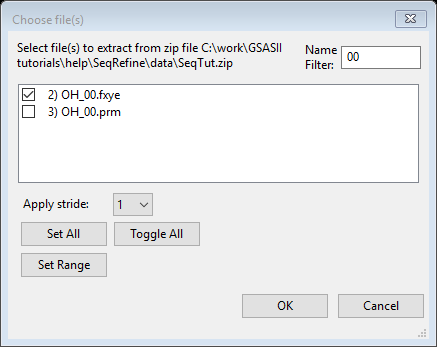
2. Read in file OH_00.fxye from file SeqTut.zip and map both phases to this dataset.
-
Read in the ~7 K dataset (OH_00.fxye) using Import/Powder Data/from GSAS powder data file
to open a file browser. Again select
“zip archive” and the SeqTut.zip file. Select file OH_00.fxye
(use of the filter can again be helpful) and press OK.
- You will be shown the first few lines from
the file. Confirm that the selected file is correct by pressing OK.
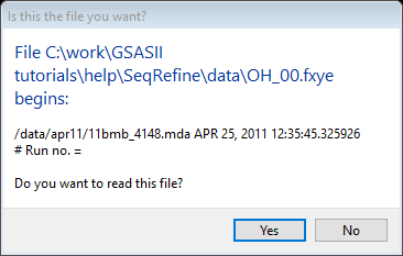
Note that the instrument parameter file with the matching name (OH_00.prm) is read automatically.
- Map the phases to the data: After reading in the dataset, a window used to select phases is shown.

Select both phases and press OK.
- Map the phases to the data: After reading in the dataset, a window used to select phases is shown.
3. Prepare for fit: define phase fraction constraint
We want to fit the lattice parameters, background, and a phase fraction initially. To illustrate how constraints are used, we will refine both phase fractions, but constrain their sum to be one. Discussion: a single powder diffraction pattern provides enough information to determine an overall scale factor and the relative amounts of each phase (with two phases: two observables), but with the scale factor and two phase fractions being varied independently, we have three arbitrary parameters, which would result in a very unstable refinement where the GSAS-II minimizer would likely remove a degree of freedom. By defining a constraint that sets the sum of the two phase fractions, we reduce this to an appropriate two parameter problem. The error of refining the scale factor and all phase fractions is made often enough that GSAS-II will warn about this and will offer to define this constraint.
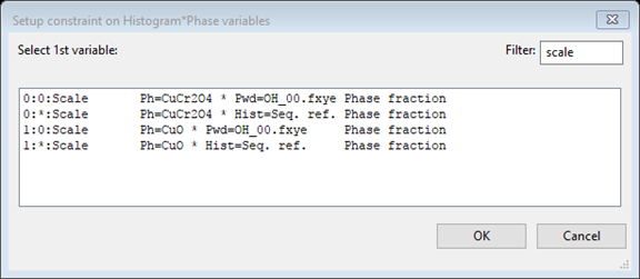
- To set up the phase fraction constraint, click on the Constraints item in the data tree and then in the Select tab menu use the Histogram/Phase menu item, and then click on the Edit Constr./Add constraint equation menu item.
- In the next window use a Filter
of scale
to make the list shorter and then select
the phase fraction for the first phase 0:0:Scale (the second one, 1:0:Scale, would work too)
- After pressing "OK" a new window
appears; in that next window either
select the other phase fraction (1:0:Scale) or select
all phases (all:0:Scale). The same result is obtained since there is only one additional
phase.

- Press OK and this creates the desired constraint, which forces the sum of phase fractions to be 1. (This is not needed here, but to change the sum and/or multipliers, press the constraint's Edit button.)
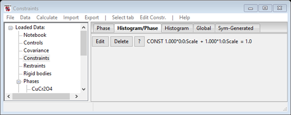
- Press OK and this creates the desired constraint, which forces the sum of phase fractions to be 1. (This is not needed here, but to change the sum and/or multipliers, press the constraint's Edit button.)
4. Initial fit: optimize lattice parameters & phase fractions; background (with 6 terms); scale factor.
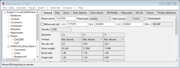
Now we select the variables to refine for each phase and then the histogram parameters.
-
Select
the first phase (CuCr2O4) click on the Refine unit
cell option (on the General
tab). (You might need to click on the triangle to the left of
the Phase
entry to “open” the tree item). We also want to refine the phase fraction for
this phase, so select the Data tab and click on the Phase fraction box to cause that to be refined.

- Repeat this with the second phase (CuO), by selecting it in the data tree. Then select the General tab and on the Refine unit cell option. We also want to refine the phase fraction for this phase, so select the Data tab and click on the Phase fraction box to cause that to be refined.
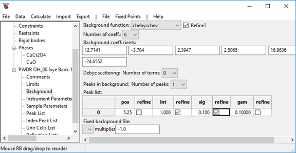
- To refine the background,
select the Background
entry under the
PWDR
OH_00.fxye Bank 1 histogram sub-entries in the GSAS-II data tree. Confirm that Background function should already
be set as chebyshev-1
and the Refine
flag should be checked. Change the No. coeff. to 6
to introduce more background terms.
- The overall histogram scale factor should already be set to be refined by default, but you may want to confirm this by clicking on the Sample Parameters data tree entry.
5. Reduce Data Range to 4.5 degrees
Finally, note that the first broad
peak at ~1.5 degrees in these data is spurious.
This artifact is known to arise from scattering from the kapton window in the
cryostat used for sample cooling; this was confirmed by collecting data without
a sample. We could model this peak, but it is easier to simply cut off the data
below the first peak at ~5 degrees. To do this, select the Limits entry for PWDR OH_00.fxye Bank 1 and in the Tmin/New
box (to lower left) change it to 4.5.
6. Perform initial fit
Use the Calculate/Refine main GSAS-II menu item to initiate the refinement. Since the project has not been saved, you will be asked to select a name (and optionally a directory) for the GSAS-II project (.gpx) file. The file name SeqTut.gpx is assumed here. The refinement progresses quickly to a Rw of ~17%.
Step II: Improve the single-temperature fit.
There are several additional variables that should now be added, now that we have reasonable starting unit cell parameters, etc. This includes a sample displacement parameter, a better background treatment and some sample broadening terms for the profile.1. Improve sample-dependent fitting.
- Refine the Sample X displacement term
- Add a background peak.
- Treat sample broadening.
Click on the Sample Parameters data tree subitem for PWDR OH_00.fxye Bank 1. Select the refine checkbox that is labeled Sample X disp. perp. to peak. The value for this is the displacement in microns (10-6 m), provided the diffractometer radius is entered correctly. Set the Goniometer radius to 1000.
Discussion: Diffractometers are never perfectly aligned, which means one should always an alignment parameter. While in older programs, the alignment parameter was a zero correction (except for Bragg-Brentano instruments), this does not properly correct for mispositioning of the sample from the center of the goniometer arc. GSAS-II offers a geometrical correction for that being offset perpendicular to the direction of the beam as the Sample X displacement (and for where data is collected to angles above 120 degrees 2theta, it is also possible to fit a second term, Sample Y displacement for displacement along the beam direction.) When using GSAS-II, refine the Sample X displacement parameter rather than the 2theta-zero correction. (Refinement of both is not normally possible).
Note: With a well characterized instrument, as is the case here for 11-BM at the APS, none of the Instrument Parameters or other Sample Parameters (beyond "Histogram scale factor" and "Sample X displ.") need to be fit.
Add a background peak at pos=5.25 degrees with int=5.0 and a sig=2000.
The background is not very well fit even with a six term polynomial due to a kapton scattering peak in the range of 4-6 degrees 2theta. This can be seen by selecting the PWDR OH_00.fxye Bank 1 tree entry and viewing the “Rietveld plot.” Then to see more detail, either press "s" to see the plot in the square-root of intensities, or zoom in so the vertical intensity scale is 0-500 counts and the horizontal region covers the first ~5 degrees in the pattern. While the fit for this could be improved by adding many more background terms, a simpler way to improve this fit is to add a broad peak in the pattern via the background fitting. This only needs 2 or 3 additional parameters.
After selecting the Background sub-item in the PWDR OH_00.fxye Bank 1 histogram, change the Peaks in Background setting from "0" to "1". Then change the peak position (pos) value to the approximate peak center (5.25 degrees) but that value should not be varied until the background is fairly well fit. Since the background generated by the Chebyschev polynomial and the background peak are highly correlated, we need to get the width and intensity into the right vicinity. Note that as the values in the peaks list are changed, the background curve (in red) is recomputed. In that way the effect of the change in values can be seen. A sig value of 2000 gives a Gaussian FWHM for this peak of ~2 degrees. Changing the int value from 1 to 5 makes the peak much easier to see and also helps start the initial fit. Set both sig and int to be refined.
Important: note that after clicking on a checkbox, one must click elsewhere in the window so that the input is recorded.
Once the background fit has been improved we can then add the position of this peak to the fit.
Refine Cryst. Size and isotropic microstrain parameters for the CuCr2O4 phase and the isotropic microstrain parameter for the CuO impurity.
It will be easier to start the sequential refinement with a good fit for the sample broadening. For the majority phase, we should consider both crystallite and microstrain broadening. For the CuO impurity, which only has a few visible peaks, refinement of more than one broadening parameter is not likely to succeed and use of either parameter should be fine. Select the CuCr2O4 phase and the Data tab on the top of the window and then select to refine the Cryst. Size and microstrain parameters. Then select the CuO phase (note that the Data tab is still displayed) and select to refine the microstrain parameter.
2. Perform additional fit
Starting an additional refinement (using the Calculate/Refine menu item) with the addition of the six new variables to the refinement improves the fit significantly visually, though the Rw value drops only to ~15.5%.
3. Still more sample parameters.
- Vary background peak position
- Use Uniaxial (010 axis) microstrain broadening for CuCr2O4
Selecting the Background sub-item in the PWDR OH_00.fxye Bank 1 histogram and click on the checkbox to refine the position (pos) value for the single background peak.
Close examination of the pattern shows that the peak widths are still not as well fit as desired. Since strain broadening seems more significant that sample broadening, we could use an anisotropic strain model. Rather than choosing the relatively complex generalized model, we can introduce only two terms with the uniaxial model. Trial and error will show that the 010 direction works best. Click on the first phase (CuCr2O4) and the Data tab and select uniaxial for the Mustrain model and change the Unique axis, HKL from "0 0 1" to 0 1 0. Select refinement for both Equatorial and Axial mustrain.
4. Perform additional fit
Starting an additional refinement (using the Calculate/Refine menu item) with the addition of two more optimized variables to the refinement improves the fit significantly visually and the Rw value drops to <14%, but the additon of the new background parameter causes issues with correlation between the background terms. Considering that we have not refined any atomic parameters, this is an very good fit despite the seemingly high Rw value, as shown in the plot below. Clicking on the Covariance data tree item shows the GOF=1.08 and the Reduced χ2=1.16. This is close to ideal. While atomic parameters could now be refined, this is clearly a good enough place to start refinement with all the datasets.
Step III: Prepare for sequential fit.
There is one significant way that sequential fitting differs from the usual refinement process. Rather than fitting lattice constants (for which there will be only one set for each phase in the entire refinement), we will use the Hydrostatic/Elastic strain terms (parameters <p>:<h>:Dij) to treat the change in lattice parameters from histgram to histogram.
More details: Note that GSAS-II shows the user unit cell parameters in the traditional a, b, c, α, β & γ (distances in Å, angles in degrees), but computations are performed internally only after converting this cell to a version of the reciprocal lattice tensor we call the "A tensor" or the Aj terms (see the GSASIIlattice documentation). The actual values refined in GSAS-II are the Aj terms, as allowed by unit cell symmetry. There is one set of Aj values for each phase, but to treat the situation where the use of a phase in each histogram may have somewhat different lattice parameters (see the PbSO4 combined fitting tutorial, where the x-ray and neutron data were collected at different temperatures), GSAS-II defines Dij terms, labeled as "Hydrostatic/elastic strain coefficients", for each phase in each histogram and only the unique terms are shown on the Phase "Data" tab. These values are simply added to the Aj terms. When any Dij terms are non-zero, the changed unit cell parameters are also shown on the "Data" tab and will differ from the unit cell values shown on the "General" tab.
1. Remove refinement of sensitive parameters (lattice, phase fractions, size/μstrain, background peak and sample displacement) and add refinement of the Dij terms.
For the initial fitting of datasets over a range of conditions, we will want to start from the fitted values we have fit, but until we have reasonably good values for the scale factor, background and lattice parameters, we do not want to refine any thing else.
-
Select the first phase (CuCr2O4) and on the General tab,
click on the Refine unit cell option to turn off refinement.
- On the Data tab (for CuCr2O4), turn off refinement of the Phase
fraction, the size and both the mustrain
parameters. Turn on refinement of the D11, D22 and
D33 terms to allow the combined lattice parameters to vary.
The Data window should look something like

-
Select the second phase (CuO) and on the
Data tab (since that is shown first), turn off refinement of the Phase
fraction and the microstrain
parameters. Turn on refinement of the D11, D22 and
D33 terms to allow the combined lattice parameters to
vary. We could refine the D13 term [which is related to
cos(β*) angle for CuO] but the changes to this are small and
since this is a minor phase and few CuO peaks are seen, it is best
to not vary this, at least initially. The Data window should look
something like

- On the General tab for CuO, click on the Refine unit cell option to turn off refinement of that.
- Also
at this stage, turn off
refinement of the background peak refinement position and width (sig)
terms by clicking on the Background histogram tree item and removing
checks from the first and third items in the background peaks table
(which has only one row). Be sure to click
elsewhere in the window before going on to the next step.

- Likewise, select the histogram Sample Parameters tree entry
and on that window, turn off the refinement flag for Sample X displ.

- At this point the refinement could be repeated to show that the fit does not change significantly. If this is done, one will see small non-zero values for the Dij terms, but the unit cell parameters displayed on the "Data" tab are not significantly different from those computed without the Dij values shown on the "General" tab, but due to the larger uncertainties on the CuO unit cell parameters, the Dij terms are much larger than for CuCr2O4.
Step IV: Import the remaining datasets.
In this step we bring in the remaining data. Note that the values for the parameters for the newly-read histograms (on the Sample Parameters data item) and the phase/histogram parameters on each phase's Data tab are set to default values, so we copy the values from the first histogram to the new sets. We can then perform an initial sequential fit.
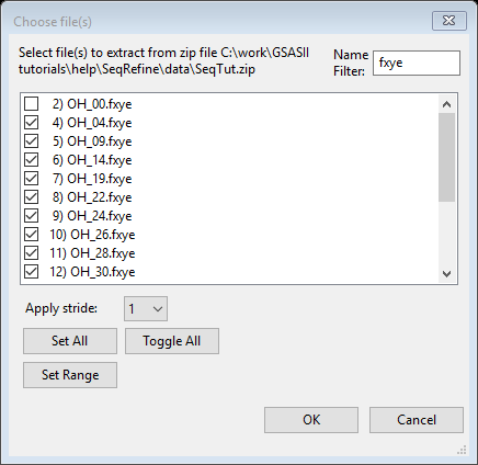
1. Read the remaining datasets.
-
Read the
remaining datasets using the Import/Powder Data/from GSAS powder data file
to open a file browser. Again select zip archive
and the downloaded SeqTut.zip file. Select all the .fxye
files except OH_00.fxye (use of the filter can
again be helpful to show just the data files; press Set All and then
unselect the one unneeded file or equivalently one can select only the
OH_00.fxye file and press Toggle All). The press OK to
start reading the datasets.
- This time one must select the
instrument parameter file (because the name does not match the dataset
file name).

- Set all data sets to use the two phases, as before in step I.2.C (above).
- Optional: Note that the default graphics
mode is to display the last dataset read in.
If you want to see the entire ensemble of data sets, click on the main
entry for any of the datasets (for example PWDR OH_00.fxye Bank 1), click on
the frame of the plot window and press the “m” key. (Alternately, press the “K” icon from the list
at the bottom of plot, between the “floppy disk” and “question mark” icons and
then select “m: toggle multidata plot” from the pop-up window). The
‘U’,
’D’,
’R’
& ‘L’
keys control the appearance of a ‘waterfall plot’.

- You can then select the ‘C’
key for a contour plot of all the data; use ‘U’ and ‘D’
keys to change the contrast.
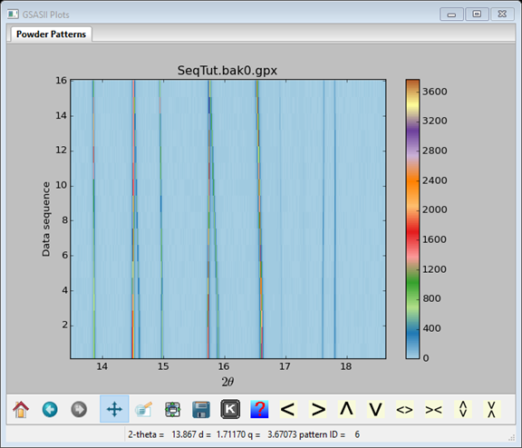
Above, I’ve used ‘D’ to increase the contrast & zoomed in to a location that shows the effect of temperature on the peak positions.
Note that the files will be processed in the order they appear in the tree (or the reverse of that order, as set in Controls). It will be most convenient if the files are imported in a logical sequence, which could require multiple Import operations to read the files in the desired order or to rename files prior to reading so they are listed in the correct order in the file browser. If files are not read in the intended order, it will be necessary to manually change the positions of the tree items (by dragging them in the tree with the right mouse button pressed). This is not an issue in this example, since the files are listed in a zip file in the order they need to be read, but may be of concern for other cases.
2. Duplicate information across histograms.
-
To copy
the histogram parameters from the first histogram to the new ones:
select the original PWDR OH_00.fxye Bank 1 tree entry and then
use menu command Commands/Copy params.
We need to duplicate the values in the Limits,
Background and Sample Parameters sections between all
histograms. The Instrument Parameters have been read from the
instrument parameter file, and have not been changed in this
exercise, so they are already identical.
This opens a dialog box where the sections to be copied are selected. Limits, Background and Sample Parameters must be selected; there will be no difference if Instrument Parameters is selected, since the parameters start as identical, so there also is no harm in copying them. This, the default entries, selecting all sections, need not be changed.
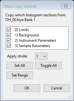
- Press OK. Note that all Sample Parameters are copied, except measurement information such as setting angles, temperature, etc.
- An additional dialog window is shown which asks which histograms should receive the parameters. Press Set All to select all remaining histograms and then pressOK.
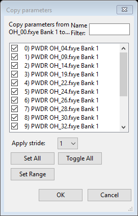
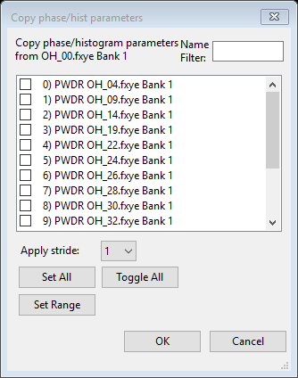
- Next we need to copy the Phase/Histogram parameters within each phase. To do this, select the first phase (CuCr2O4) in the data tree and then the Data tab in the window. Then use the Edit Phase/Copy data menu command, which raises the selction window below.
- Repeat the previous step for the CuO phase. Select CuO in the data tree and then copy the Phase/Histogram parameters in its Data tab by again using the Edit Phase/Copy data menu command. Again, select all histograms and then press the OK button.
To verify that the copy has been performed, examining any of the other histogram plots (e.g. to see the changed lower limit), etc. or view the contents of the various updated sections.
Press the Set All button and then press the OK button.
Step V: Setup and start the sequential refinement.
At this point we determine which histograms will be used in the fit and set that the resulting parameters from the results of each refinement will be used for the subsequent refinements.
1. Set overall Controls for a sequential fit and launch it
Here we enable sequential mode by setting the histograms to be included, set another control setting (max cycles) and launch the sequential fit.
-
Select the Controls data tree item, in the window (as shown
below) and press the "Sequential Refinement
Select data" button.
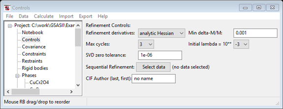
This opens the window where all histograms can be selected. Press Set All and then press OK. Note that the Controls window now lists the number of datasets in the sequential refinement and three new controls below that. One is the new "Reverse order?" checkbox, which causes the sequential refinement to start with the last histogram, not the first. Sometimes this is useful, but not here. The "Clear previous seq. results" will remove previous sequential results from a .gpx file, reducing its size. The "Copy results to next histogram?" is described in the next section.
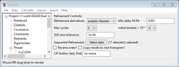
- Important: Check the "Copy results to next histogram?" checkbox. When this is selected, the parameters obtained after fitting each histogram will be used as the starting point for the next fit, which is essential here since the lattice parameters change considerably. If this were not selected, then refinement for each histogram would start with the current parameters for that histogram -- these were obtained from fitting the first (~7 K) dataset. If we did that the first few refinements will go well, but when reaching datasets where the temperature was sufficiently different from 7 K, the starting lattice parameters may be too far off and the refinements will fail. Even if that were not true, since the temperatures are fairly close between datasets in the series, each fit will start with a fairly close to correct set of lattice parameters and thus fewer cycles of refinement will be needed to get to the correct values.
- Also on the Controls window, change the Max cycles setting to 10. This makes sure that the refinements have enough cycles to fully adjust to the changes in lattice parameters before being used as the starting point for the next refinement. Note that if the refinement converges, no additional cycles are used, so 10 is a maximum that is not likely to be reached.
2. Start the sequential refinement
Start the sequential refinement with the Calculate/Sequential refine menu command (note that once the histograms were selected for a sequential fit in the previous step, the menu command was relabeled from Calculate/Sequential refine.)
Note that a window saying "There were constraint warnings..." will be generated. This is because we have specified a constraint on the phase fractions in step I.3, but we are no longer varying them, so this constraint must be ignored. Also note the discussion on sequential fit constraint modes in step VI, below. This alert is shown to provide a chance to review possible problems with constraints and not continue with the fit, when this indicates that something has been left out from the varied parameters. However, in this case, this phase fraction constraint will be fine to ignore since we do not want to refine phase fractions at this stage. This message will stop being shown when phase fractions are refined again (or if the constraint would be removed). Press "Yes" to continue with this initial sequential fit, as this warning can be ignored.
The refinement may take a few minutes as each of the 17 datasets are fit in turn.
3. Accept the sequential refinement results.
When the refinement completes, a window will be displayed where you are asked if you want to load the results, as below.

After clicking on OK the Sequential Results item is created in the data tree and is is selected, which displays a summary of the refinement results as a large table, as below.

The second column shows the weighted profile R-factor, from each fit. This shows a steady increase with temperature, as might be expected if there were a systematic change in some sample parameters, such as strain or background or even atomic coordinates (which have not yet been fit). The Δχ2 value in the third column shows the percent improvement in χ2 seen in the last cycle of refinement. (Meaning that if in that cycle the Δχ2 value decreases from 4.1 to 4.0, then the value will be 100*(4.1-4.0)/4.0, or 2.5%; small numbers indicate that the fit converged.). Note that the fits had pretty well stopped improving, so there is no reason to provide further cycles of refinement without adding new variable parameters.
Subsequent columns will show any of the sample parameters that vary across the datasets, here only temperature and then the direct cell lattice constants for each phase, generated from the Ax and Dij terms. Scrolling further shows columns the values of most parameters that differ by histogram. Note that some parameters (such as the actual Dij terms) are not shown. The choices for which items that are included is determined by the "Hide columns..." command in the"Columns/Rows" menu.
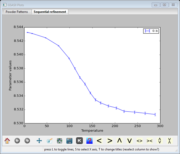
4. Examine the sequential refinement results.
Before going further, it is useful to review the trends in the lattice parameters as a sanity check. This can be done by double-clicking on a column of the table, such as the 0::b parameter, which displays this plot:
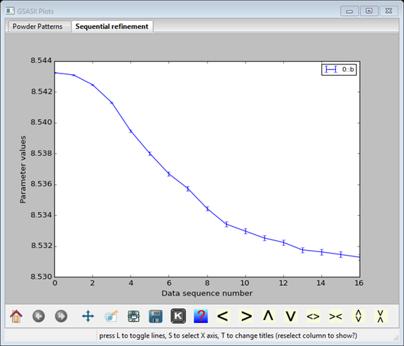
Pressing the “K” icon or pressing the “s” key brings up a menu where the x-axis can be selected as Temperature. If the plot fails to update, click on another column and then return to the original column.
Step VI: Continue the sequential refinement.
At this point we wish to continue the refinements using the the current as-refined parameter values as the starting point. This is the default action for the program as the Copy results to next histogram checkbox is automatically unchecked after a successful sequential refinement. Note that in subsequent actions we will use the "Copy flags" menu commands, which copy only refinement flags not parameter values (as opposed to the "Copy" commands used previously, which copy both values and flags.)
1. Restore the parameters that were previously fit.
- Restore the refinement of background parameters as in the single-histogram fit. Select Background for any histogram and add the "Peaks in Background" width (sig) refine flag. Note that the peak position could be refined as well, but this is not well-determined by the data since very little of the low-angle side of the peak is present, so inclusion of this adds to the refinement instability without any significant improvement to the fit.
- After setting the refinement flag, use the Background/Copy flags menu item to copy these refinement flags to all other histograms.
- Likewise, in the Sample Parameters tree item, include the Sample X displ parameter and again use the Copy flags menu command (here in the Command menu).
- For the CuCr2O4 phase, return to the Data tab and enable refinement for the phase fraction and the three broadening terms (isotropic size and equatorial and axial mustrain). Again use the Edit Phase/Copy flags menu command to set these flags for all histograms.
- For the CuO phase, also on the Data tab, enable refinement for the phase fraction and the single isotropic microstrain broadening term. Also add refinement of the D13 term. Again use the Edit Phase/Copy flags menu command to set this for all histograms.
- Select the Constraints data tree item and note that the second line of controls that appears for sequential fits. Confirm that the "Wildcard use" setting is "Set hist # to *".
Note:
Refinement of phase
fractions requires a constraint as was added in Step
I.3, but for all histograms.
As of version 5038 of GSAS-II three modes were added for constraints
in sequential refinements.
"Ignore unless hist=*" mode (which was
the only mode prior to this version), any constraints with a
specific histogram number specified (such as ":0:0:Scale" and
":1:0:Scale" as used previously) would be ignored and a new
constraint defining ":0:*:Scale + :1:*:Scale = 1" would be
required.
2. Perform the refinement.
Start an additional refinement (using the Calculate/Refine menu item). Now that the full suite of variables is available for fitting background, peak widths, etc., the fits improve significantly for the higher temperature datasets. Before, for the highest temperature datasets, the Rwp values were in the range of 25-30%. After this fit, all the Rwp values range from 13-17%. Click on a row header to see a plot of the fit and double-click on a row header to see the convariance matrix plotted. Note that additional columns appear now in the Sequential results table for the newly-added variables. Also included are the weight fractions. Note that the sum of the phase fractions for each histogram are indeed 1.0.
Step VII: Complete the sequential refinement.
The last thing we will add to the refinement will be atomic parameters. Note that these are handled a bit differently than the previous things we have refined. There is only one set of coordinates for each phase and these will be refined for each histogram, but are saved individually only in the Sequential results table. To update the coordinates shown in the Phase data tree entry, use the "Update Phase from selected" command in the"Columns/Rows" menu. If a row is selected in the table, that will be used. If no rows are selected, you will be prompted to select a histogram.
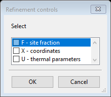
1. Vary CuCr2O4 coordinates and Uiso Parameters.
- Select the CuCr2O4 phase and then the Atoms tab. Double-click on the refinecolumn label and a refinement controls dialog opens as below, select X to refine coordinates and U to refine the atomic displacement (Uiso) values. (Note that only the O atom has coordinates that can be refined, all coordinates for Cu and Cr are fixed by symmetry. Use of the X flag for Cu and Cr will not cause those coordinates to change.)
- Note the change that appears in the refine column of the atoms table, as below. Since these parameters are shared in all histograms, no Copy or Copy flags menu item is needed or even is available for atomic parameters.

2. Perform final sequential fit, including coordinates displacement parameters.
Start the sequential refinement again with the Calculate/Sequential refine menu item. Small but significant improvements are seen for fits with the higher temperature datasets, with Rwp values between 13.8 and 16.5.
This completes the sequential refinement tutorial, although a few more things could be attempted to try to further improve the refinement quality. Be sure to keep the final project file, since this will used in the Parametric Fitting and Pseudo Variables for Sequential Fits tutorial, where functions of fitted parameters are computed and plotted and these results are fitted to equations of state.