Rietveld Fitting with Rigid Bodies

Introduction

It is a common situation that a powder diffraction dataset will not provide enough observations to allow refinement of all atoms independently. This is not only a problem for powder diffraction; it is usually the case in single-crystal protein structure determination as well, as few datasets for that can be collected to atomic resolution. When the number of parameters is not sufficient to discern individual atomic positions, it is necessary to apply constraints and/or restraints. Constraints simplify the crystallographic model by reducing the number of parameters. Restraints treat assumptions about the model as experimental observations.  Examples of restraints include providing target values for bond distances and angles, or penalizing a refinement if atoms diverge from a plane. One common constraint is to group U_iso values so that a single value is used for all atoms of a particular type or in a common bonding environment.

One of the more powerful types of constraints in GSAS-II is to constrain a group of atoms so that their relative positions are fixed. Such a group of atoms is known as a rigid body. The core concept behind rigid body refinement is that 3 parameters define an origin and only 3 orientation parameters are needed to locate a rigid body, so that only 6 parameters are needed to locate and orient the body, though in some cases symmetry will constrain some of these values and the number of refinable parameters will thus be reduced. In contrast, 3 position parameters are needed for every atom in a structure on a general position. Thus, a four-atom group requires 12 positional parameters and a 6-atom group requires 18 positional parameters, when modeled with individual atoms, but as rigid-bodies only 6 parameters will be needed. Also, since the relative positions are fixed, rigid bodies result in a more chemically reasonable structure.

GSAS-II offers two types of rigid bodies. This tutorial will demonstrate use of one type, residue rigid bodies, which allow incorporation of optional torsional parameters. The second type, vector rigid bodies, offer one or more refinable size parameters, which can allow for refinement of selected bond distances or geometrical factors, but this is less commonly needed, compared to torsions.

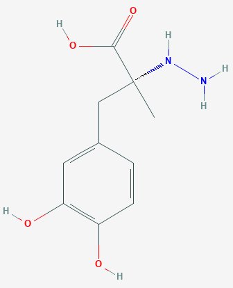
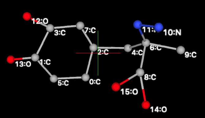
In the supplied example GSAS-II project file, a powder diffraction dataset is supplied for a sample where there are two independent copies of the chiral R-(+)-Carbidopa molecule (shown below) as well as two water molecules in the asymmetric unit.

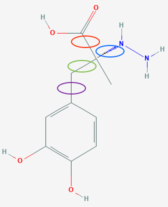
Since chemical knowledge dictates that the 6 atoms in the phenyl ring, as well as the 6 atoms bonded to them, will lie in a plane, and since bond distances and angles are well known for those atoms, there is no reason to give these atoms any degrees of freedom in the model used to fit the diffraction data, beyond the orientation and position of the group. The positions for the remaining non-H atom can be determined with only 4 additional parameters, noting that rotation is possible around the four bonds circled below.

Thus, all 16 non-hydrogen atoms can be positioned with 10 parameters: 3 coordinates, 3 orientation parameters and 4 torsions. This is almost a five-fold simplification compared to the 48 positional parameters needed for 16 unconstrained atoms. If we had neutron data that would allow location of hydrogen atoms, adding 5 more torsions would allow for the hydrogen atoms to be positioned as well, where a total of 30 atoms would be located from 15 parameters.

In this example, the fit in the supplied GSAS-II project file appears quite good with respect to the agreement to the observed data, but closer examination shows that the bond distances and angles of the two molecular groups are quite irregular. Since this distorted structure is not physically reasonable, this model is not acceptable. This well-fitting but poor-quality model arises because too many parameters were introduced, which is sometimes called overfitting. In this tutorial, a better model will be developed using rigid bodies for the two molecules, providing a more chemically reasonable representation with fewer parameters -- simply a better fit.

Step 1. Export Cartesian coordinates for R-(+)-Carbidopa from a crystal structure

There are two steps to working with rigid bodies in GSAS-II. The first is to obtain an accurate set of coordinates for the molecule, molecular fragment, or ionic moiety, which can be done in a number of ways. One way is to locate an accurate crystal structure from a database or paper. A second method is to use a computational tool to determine an approximate structure regularized for reasonable bond lengths. This can be done with low-accuracy forcefield computations or varying levels of improved theory. A good tool for simple forcefield minimization is the free cross-platform Avogadro program.

Note that we could generate the R-(+)-Carbidopa fairly simply from inside Avogadro by drawing the molecule (process described here), or even quicker, since the PubChem entry lists a SMILES description of the atomic bonding [C[C@@](CC1=CC(=C(C=C1)O)O)(C(=O)O)NN], that description could also be used using the Avogadro Build/Insert/SMILES… menu command, but in this step we will use a more general method to input a molecular fragment to Avogadro, so that it can be regularized.

1A) For this tutorial, we will export coordinates from GSAS-II in a form to be read Avogadro. They will be regularized in the next step.

Begin by starting GSAS-II. Any .gpx file (GSAS-II project) may be used. If a new, empty, project is used, select the Data/“Add new phase” menu item first. Select the Rigid Bodies tab in the data tree.

1B) Use the “Edit Vector Body”/“Extract from file” menu item select the GSAS-II gpx format and read in the distort1.gpx file included in the sample input. This will read in the coordinates for 34 atoms (two carbidopa molecules and two O atoms), from this we want to select only one carbidopa molecule.

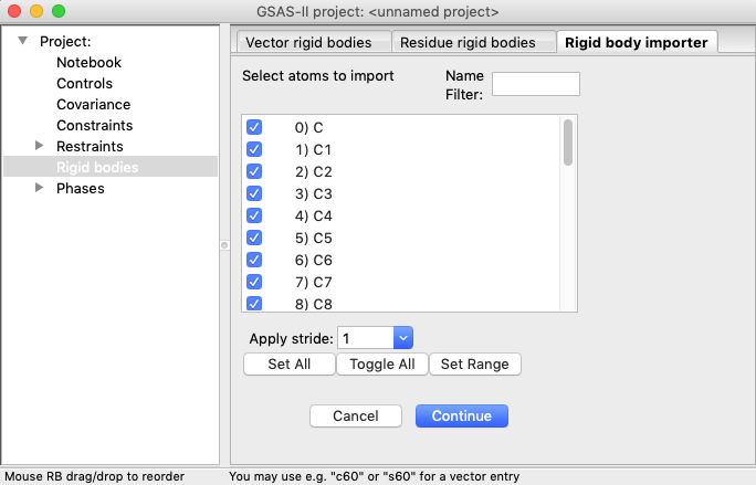
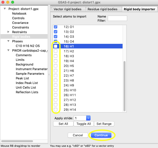
1C) Unselect all atoms by pressing the Toggle All button and then select the first sixteen atoms using the “Set Range” button and selecting the first [“0) C”] and the sixteenth atom [“15) O3”]. Note that in the plot of the structure, unselected atoms appear partially “greyed out” compared to selected atoms.

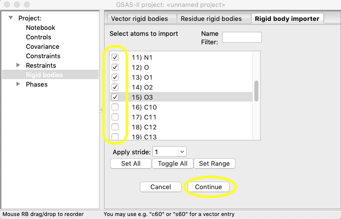
Once the 16 atoms are selected, press “Continue”. The rigid body then appears in the plot window. Note how distorted the molecule appears.

1D) If these coordinates were satisfactory, the rigid body could be created at this point, but since these coordinates are distorted, we will regularize them in Avogadro first. Export the coordinates by pressing the “export as xyz” button on the GSAS-II window.

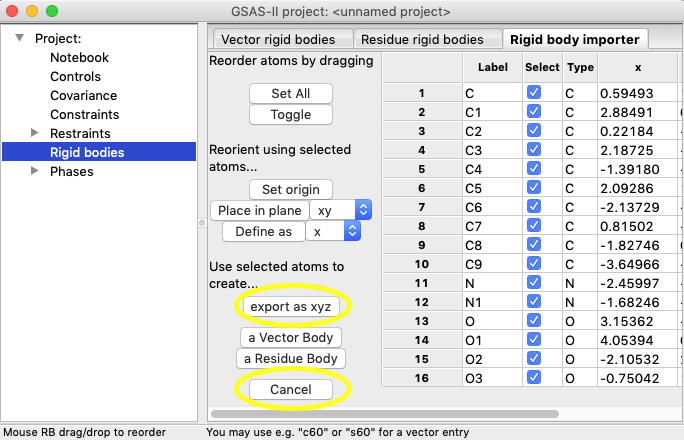
Make a note of the file name, as it will be needed in the next step. Press Cancel to close this window. It is fine to close GSAS-II, but it can also remain open.

Step 2: Regularize coordinates in Avogadro

For this step, it is assumed that the cross-platform software Avogadro program has been installed. If you do not want to install this program, this step can be skipped, as described at the beginning of Step 3.

2A) Read the coordinates into Avogadro by starting the program and using the Avogadro File/Open command; select the XYZ file type option and read the file produced in step 1D.

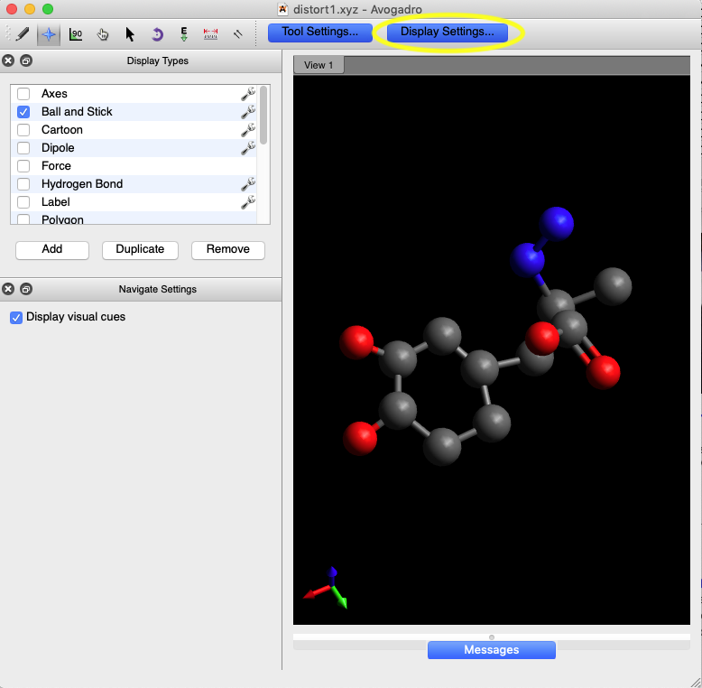
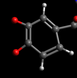
2B) Note that the program noted the correct bonding of the carboxylic acid group, where one of the C-O bonds is noted as a double bond, but the phenyl group does not have alternating double bonds. To fix this, we need to click on the bonds, but that is difficult to do unless the atoms are drawn smaller. Make sure that the Display Settings button is selected (at top of window) and click on the wrench symbol to bring up the “Ball and Sticks Settings” dialog, below.

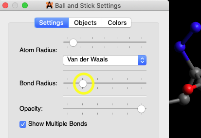
When the “balls” are made smaller by moving the Bond Radius slider to the left, it becomes possible to click on bonds.

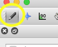
2C) Switch to the pencil in the toolbar

Click on directly on every other C-C bond in the phenyl ring to change the bonds from single to double. Note that when a C-C bond is clicked on, the order changes successively from single to double and to triple and then back to single again. (Use care to avoid clicking elsewhere than on a bond or additional atoms will be created; use a right click to delete unneeded atoms.)

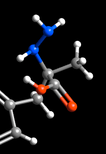
2D) Use the Build/“Add Hydrogens” menu item to add the remaining H atoms to the other end of the molecule.

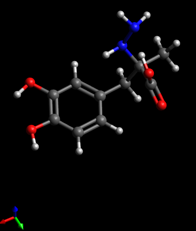
2E) Optimize the bond distances and angles using Extensions/“Optimize Geometry”. Use it a few times until no further changes are visible. The molecule should appear as below, with regularized bond distances and angles.

2F) Use “Save as” to write the newly generated coordinates out. Be sure to select the file type as “XYZ”. I used the name regularized.xyz for the file. Exit Avogadro.

Step 3: Create the rigid body in GSAS-II

If you skipped step 2, you can use the file I created with Avogadro, supplied as regularized.xyz in the Exercise files.

3A) To start, in GSAS-II open the distort1.gpx file that is supplied in the Exercise files. We then will create a rigid body for this project. Start by clicking on the “Rigid bodies” tree item. Click on the “Edit Residue Body”/“Extract from file” menu item, select the format as XYZ and then select the file written in step 2F (regularized.xyz).

Note that the “Import XYZ” menu command could also be used, but “Extract from file” allows atoms to be selected, recomputes the origin as the midpoint between atoms and allows rigid body axes and the origin to be defined based on user preferences. With “Import XYZ” the coordinates would be used exactly as in created by Avogadro.

3B) After the regularized.xyz file is opened and read; all atoms are selected by default. Note that H atoms are not moved when torsional groups are rotated, so we do not want to include any of the non-phenyl H atoms. For simplicity, here we will remove all of the H atoms. (They could be regenerated later, if desired). Select only atoms #0-#15 (as below) and press Continue.

3C) Note that there are several other things that can be done on the window that is now created. These include: defining axes and reordering the atoms by dragging rows in the list. As an example, selecting the atoms in the phenyl ring and pressing “Place in plane”, where the adjacent button has “xy” selected, will orient the z axis as normal to the plane of the ring. Selecting a single atom and pressing “Set origin” will place that atom as the origin, or if two atoms are selected the origin will be the midpoint between the two atoms. None of this is needed here, but such actions will likely be needed for bodies that will be placed at high-symmetry locations in a unit cell.

For this exercise all that is needed to select all atoms (done by default) and then use the selected atoms to create a rigid body by pressing the “a Residue Body” button near the bottom of the list of buttons.

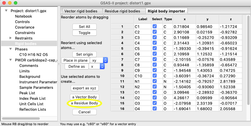
The rigid body is then created as shown below.

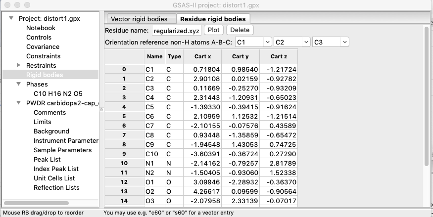
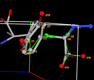
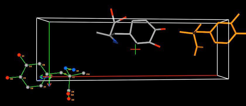
3D) Find atoms in torsions

Press the Plot button to see the rigid body. Note that dragging with the left mouse button held down is needed to see all the atom labels, as below.

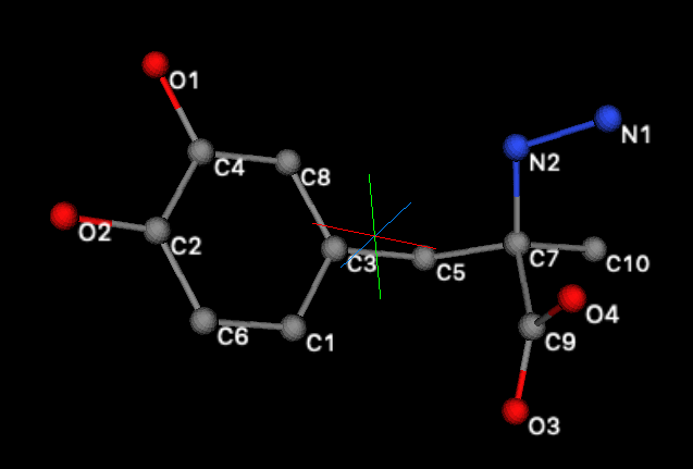
From this it can be seen that the four bonds with possible torsional rotations are:

a)    C3-C5,

b)   C5-C7,

c)    C7-N2 and

d)   C7-C9.

3E) Define the torsions

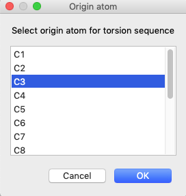
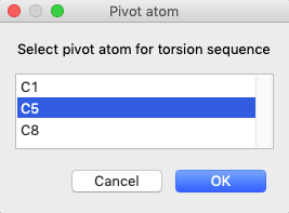
Press the “Edit Residue Body”/”Define torsion” menu item. This opens a window to select an origin atom. Once that is selected, you are offered a choice of atoms that are bonded to the selected atom. Thus, for the C3-C5 bond, select C3 first to be the origin atom and press OK. This will open a second menu with options for the pivot atom: C1, C5 or C8. Select C5. (Note that if C5 had been selected first as origin, then the pivot choices would be C3 and C7.)

After defining the C3-C5 for a torsion, repeat this to define a total of 4 torsions, by adding C5-C7, C7-N2 and C7-C9. The torsions are displayed at the bottom of the window, as shown below:

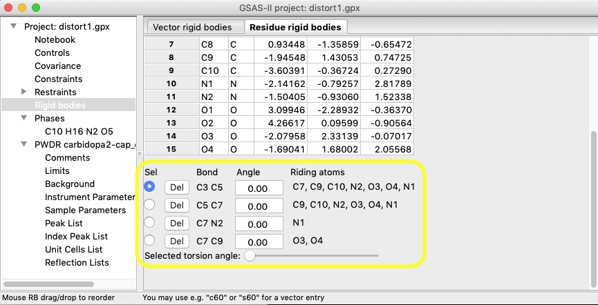
It can be instructive to select each torsional mode in turn and move the slider to see how the mode rotates the riding atoms.

Introduction to Steps 4 & 5

Now that the rigid body has been defined, the next step is to insert it into the crystal structure model. This means defining where the rigid body is located, oriented and how it is mapped to atoms in the asymmetric unit. The origin of the rigid body Cartesian system is placed at a specified location (in fractional coordinates) and a quaternion defines the rigid body orientation. The same rigid body may be inserted multiple times in the asymmetric unit. Each insertion of each body will have a corresponding set of atoms in the asymmetric unit, an origin, a quaternion for orientation. There will also be a set of torsion angle values associated with each body insertion.

Note that understanding GSAS-II’s 3D visualization system is key to managing rigid bodies. It is valuable to move and rotate the representation, so that distances along all axes can be visualized. For this it is valuable to understand that as the structure is viewed, movement of the mouse while holding down a button (also called dragging) changes the view of the crystal structure, as described here:

·      Dragging with the right button down: moves the viewpoint, which is kept at the center of the screen (effectively translating the structure).

·      Dragging with the left button down: rotates axes around screen x & y. Rotation is around the viewpoint.

·      Dragging with the center button down: rotates axes around screen z.

·      Rotating the scroll wheel: changes “camera position” (zoom in/out).

Note that the screen axes are x: horizontal; y: vertical; and z: out of screen. Also, there are additional plot controls available by pressing on the “Draw Options” tab.

When inserting a rigid body into a unit cell, as described in the next section, as the rigid body is being located into the unit cell, a second set of actions can be accessed with the mouse that affect the rigid body positioning. This is done by holding the Alt keyboard key down while “dragging” the mouse.

·      Alt+right mouse dragging moves the rigid body by shifting the origin.

·      Alt+middle button dragging rotates the rigid body around the screen z axis.

·      Alt+left button dragging rotates the body around the x & y screen axes.

Visually, the rigid body motions are analogous to what appears when the view of the structure is changed.

In this tutorial, we want to place the rigid bodies into the approximate locations where those molecules are already found. There are two ways to do this. One is that if specified atoms in the rigid body are paired to atoms in the crystal, the origin and/or quaternion can be optimized to best collocate those pairs of atoms. This will be shown in Step 4. Another choice is to visually move the rigid body to the desired location, which will be shown in Step 5. That process might be needed to insert a molecule into a specific region of a structure to fill a void or to account for density in a Fourier map.

Step 4: Insert the first rigid body into the model

In this step we will assign matching pairs of atoms between the rigid body and the crystal asymmetric unit and use them to determine the rigid body location.

4A) To start the process of inserting a rigid body into a structure, select the desired phase in the data tree (here there is only one choice) and then select the “Edit Body”/“Locate & Insert Rigid Body” menu item. If more than one body were defined, a window to select which body would be offered. A farily complex window is displayed with options to define where the rigid body will be placed, as below.

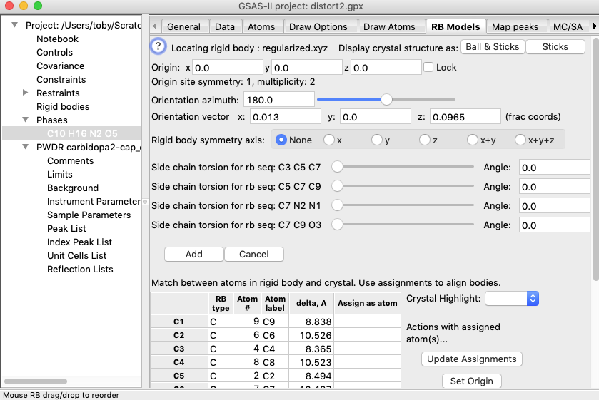
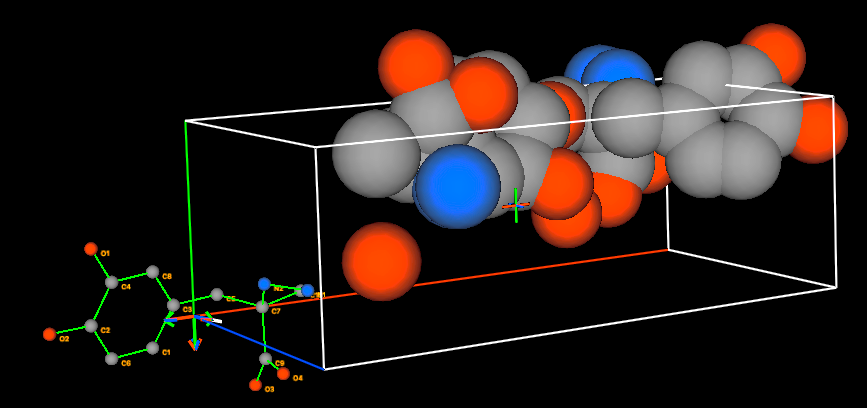
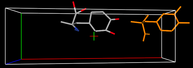
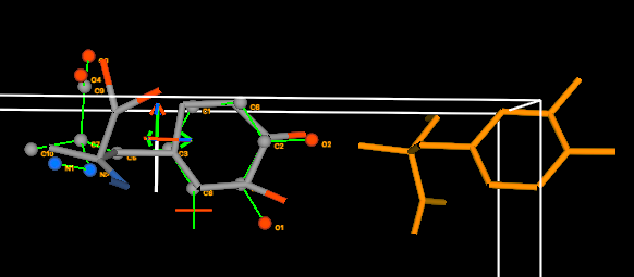
Also shown in the GSAS-II graphics window is a plot of the structure, along with the rigid body location. The structure will be plotted as was set in the Draw Atoms tab. Note that here, by default, the asymmetric unit is shown with van der Waals spheres. The rigid body is always displayed as a ball-and-stick model with green bonds. Note that the origin of the rigid body is shown with a triplet of red, green and blue lines (for x, y, & z, respectively). A white line is also shown that displays the orientation vector. The red, green and blue lines (for x, y, & z, respectively) of the unit cell outline show the origin and axes of the crystal. The same color sequence show these axes on the viewpoint.

Change the crystal structure display mode to either Ball & Sticks or Sticks (your preference) using the buttons on the upper right. This is needed because with van der Waals spheres, it is hard to see when the rigid body is close to the location where it will be docked.

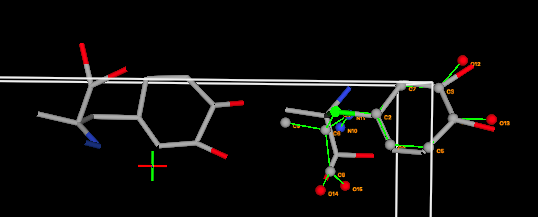
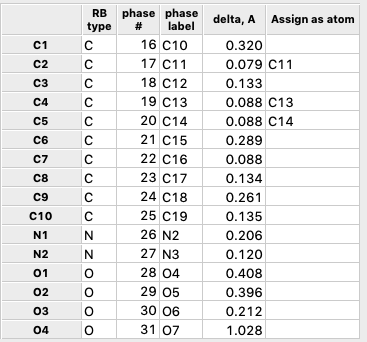
Note that the table at the lower part of the window (as seen below) shows each atom in the rigid body and the closest atom in the crystal structure as well as the distance to that atom. In the column labeled as “Assign as atom” to the extreme right of the table, we can assign specific pairing between atoms in the rigid body and atoms in the crystal structure that will override the closest atom pairing. As the rigid body is moved, the distances will be updated. Unless a pairing assignment has been made, the closest atom pairing may change as the body moves.

4B) We will align the rigid body to the molecule in the cell closest to the upper right corner by assigning rigid body atoms to the matching atoms in the unit cell. Scrolling or expanding the window so the entire table is visible will make subsequent steps easier

If we click on the 2^nd row in the table (with row label “C2”), the row is highlighted.

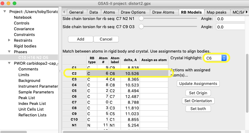
Note that atom C2 in the rigid body is highlighted by the ball color changing to green, as well as its paired atom in the crystal structure (C6), as shown below.

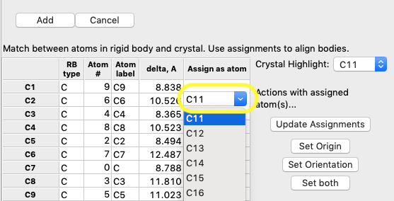
The crystal structure atom is not the correct one to match to C2. To find the right one, we can highlight different atoms in the crystal structure by pressing the Tab keyboard key until the correct atom is displayed; alternately, select different atoms in the “Crystal Highlight” pull down. After cycling through, one can see that C11 in the crystal structure should be paired to C2 in the rigid body.

4C) Assign C11 in the crystal structure to be paired to C2 by clicking in the right-most box in the C2 row of the table and selecting atom C11 from the dropdown list, as seen below.

Optional: press “Update Assignments” button and the distance between RB C2 and unit cell C11 will be shown in the table. Likewise, pressing “Set Origin” will translate the rigid body to best match the assigned atoms. Since there is only one assigned atom, the distance will be zero.

4D) Setting the orientation and origin requires assignment of at least two more atoms and preferably more. Select another easy to identify an atom in the rigid body by clicking on the C4 row in the table. (Alternately, press Alt-Tab to highlight different rigid body atoms.) Using Tab, it can be seen that crystal structure atom C13 should be paired to RB atoms C4. Select atom C13 in the “Assign as atom” cell for C4.

Likewise, rigid body atom C5 should be assigned to crystal structure atom C14 by selecting atom C14 in the “Assign as atom” cell for C5.

4E) Then press the “Set Both” button and the phenyl ring positions are approximately matched, as below.

4F) The agreement in atom positions at the other end of the molecule is still not very good, and this can be improved by repositioning the view (dragging with the left mouse button) to look approximately along the plane of the ring. When this is done, it becomes clear that the agreement can be improved significantly by rotating around the first torsion angle by moving the slider. An angle of ~23 degrees brings the atoms much closer, but there are still atoms as much as 1 Å in disagreement, since the molecule in the crystal structure is rather distorted.

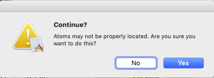
4G) Note that the table now shows that the rigid body has crystal structure atoms 16-31 paired. The pairing is consecutive, which is to be expected since the ordering of atoms was never changed, but this is not required.  Press Add to insert the rigid body, using the parameters shown in the window. A warning is displayed, since some of the distances are larger than 0.5 Å, but press Yes since this is about as good as we can do.

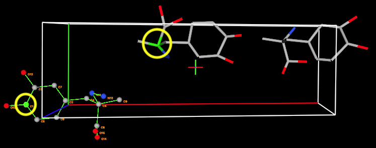
Pressing Add causes any unpaired (shown as “create new”) to be added to the Atoms list and then every atom in the rigid body is linked to an atom in the asymmetric unit.  The rigid-body constrained atoms are now shown with bonds in orange (unless “Show Rigid Bodies” is unchecked on the “Draw Options” tab.) The atom coordinates are shown with a grey background on the Atoms tab. Press the c key (with the graphics window active) to see the view below.

Step 5: Insert the second rigid body into the model

As mentioned in the introduction to steps 4 & 5, above, holding a mouse button down (mouse dragging) changes the view of the crystal while holding Alt down while dragging the mouse, repositions the rigid body within the cell. In this step, to show how that works, we will use the mouse to place the rigid body.

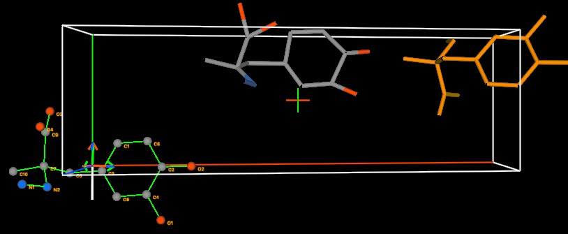
5A) To insert the rigid body into the structure again to match the second copy of the molecule, again select the “Edit Body”/“Locate & Insert Rigid Body” menu item. A window is displayed as before with options to define where the rigid body will be placed. The graphical display will look like this:

5B) Hold the Alt key down and drag with the middle mouse button to rotate the rigid body by 180 degrees, as shown below.

5C) Again with the Alt key down, drag with the right mouse button and move the rigid body so that the phenyl rings are more or less aligned.

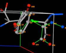
5D) To see how far the rings are separated in the screen z direction, we must rotate the view. Drag the mouse upwards with the left button down (without pressing Alt) to obtain a view similar to the one below.

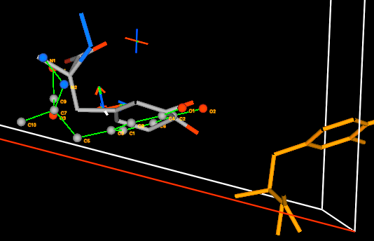
From this view it is clear that both a small rotation and a small translation is needed. First with the Alt and the middle mouse button both pressed, drag upwards until the two rings molecules are more parallel. Then, with the Alt and the right mouse buttons both pressed, drag upwards until the molecules are better overlapped.

5E) At the point the rigid body is pretty close to the position of the molecule in the unit cell, with distances in the table ranging from 0.1 to nearly 2 Å, but better agreement can be obtained by making small adjustments with the Alt down and successively pressing each of the three mouse buttons alternated with changing the view to see the molecules from a different perspective. Another choice is to assign several atoms and optimize, as was done in steps 4D and 4E. Choices of atoms to optimize are clear, since the atoms are properly paired in the table. Updating the C3-C5 torsion to ~20 degrees will also improve the agreement.

5F) When the agreement is sufficient, press Add, accept the warning and this molecule is also now constrained by the rigid body. Now both molecules will appear as orange.

Step 6: Optimize the model

If the number of cycles is set to zero (in the Controls tree item), the fit will be seen to have gotten significantly worse, with the profile wR jumping from 2.2% with the distorted model to ~6%. This is not surprising and only a few refinement steps will provide a more realistic model with comparable agreement, but far fewer parameters.

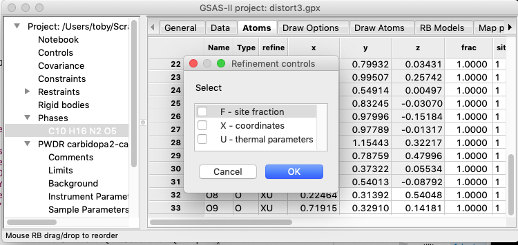
6A) Initially, turn off refinement of all atoms. (Select the Atoms tab, double-click on the refine column label and then leave all boxes unchecked and press OK). Note that the X flag for the atoms in the rigid bodies would be ignored anyway.

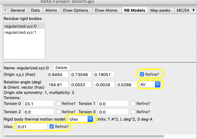
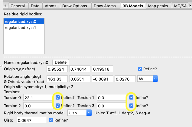
Then select the RB Models tab. The first rigid body is automatically selected. Make the following changes:

1.    Select to refine the Origin

2.    Refine both the orientation azimuth and vector by setting the AV flag

3.    Set the “thermal motion” mode to Uiso

4.    Set the initial Uiso value to something reasonable, say 0.01

5.    Set the refinement flag for thermal motion

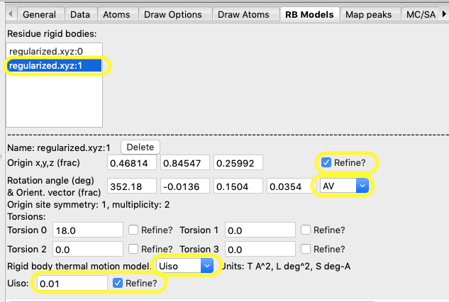
6B) Then select the second rigid body and repeat the previous actions (setting the refine checkbox, selecting AV for the orientation refinement, setting Uiso mode, set the Uiso value to 0.01 and set the thermal motion refinement flag.)

6C) Set the number of cycles back to 5 and refine. The fit will converge quickly to an wR of ~4%.

6D) Add refinement of the four torsion angles for each of the two rigid bodies. Then refine again. The wR quickly drops to 2.5%

Optional Step 7: Try rigid body TLS motion

The motion of rigid bodies, known as the TLS description, has been worked out (Schomaker & Trueblood, Acta Cryst. B24, 63-76, 1968) and consists of three tensors:

·      the T tensor for translation movement of all atoms together

·      the L tensor for libration, rotation of all atoms as a unit around the rigid body origin, and

·      the S tensor, to describe correlated librational-translational motion (screw-like motion). The S terms can be readily omitted if the rigid body origin is at the body center of mass.

In the full expansion there are 6 T and 6 L and 8 S terms. It is unlikely that all of these terms can ever be used with a powder dataset.

The simplest description that can be made with a rigid body is to assume that all motion is translational and isotropic. This is what we have done previously and is equivalent to refining Uiso for each atom in the rigid body, but applying a constraint so that all atoms in the rigid body share that Uiso value. It makes sense to see if further expansion of the rigid body motion/disorder description will produce an even better fit, although it is clear that the crystallographic fit is already quite good considering the limited resolution and high background levels. Refining 24 more parameters (6 T + 6 L, for each of the 2 bodies) is clearly impractical. One possible simplification would be to refine only the diagonal T & L elements (which constraints translation and libration directions to crystal axes). That might be appropriate with data more sensitive to group motion, but is still impractical here. One still simpler model is to include translation and libration, but require equal amplitudes in all directions. This can be done by refining only the diagonal T and L terms, but to constrain them to be equal. If the T & L values are constrained to be the same for the two rigid body insertions, this means replacing the 2 grouped Uiso values with 2 terms (a single T_jj and a L_jj term applied to all rigid body atoms). This is easily done as shown below.

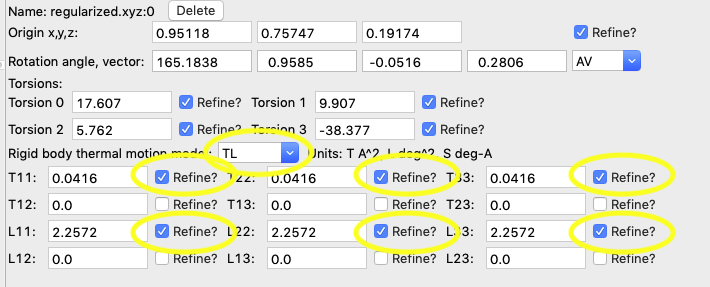
7A) Switch to refine the T & L terms by selecting each body, in the RB Models phase tab, set the thermal motion model to TL for both rigid bodies and then turn on the refine checkbox for the T11, T22, T33, L11, L22 & L33 terms. 

7B) Delete the two existing constraints on Uiso values: Use the Constraints tree item and the Phase tab and delete the two entries. These constraints are actually ignored when rigid body group motion is refined, so the presence of these constraints does not actually have any effect, but it is better to remove any unused constraints.

7C) Create constraints on the T_jj and L_jj terms through use of the Constraints tree item. To constrain the T_jj terms, one needs to know their variable names are RBRTjj:b:0 for body #b of type 0 where j = 1, 2 or 3.

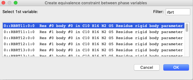
On the Phase tab (loaded by default), use the “Edit Constr.”/“Add Equivalence” menu item and enter RBRT in the search filter. The first term is one of the six that needs to be constrained, so select it as the 1^st variable and press OK.

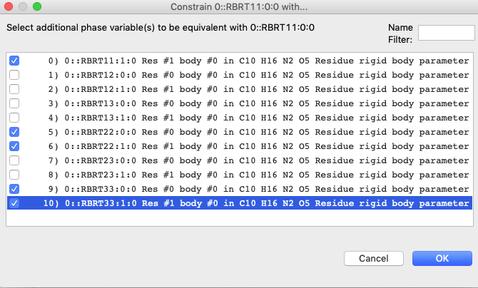
On the next window select the remaining five 11, 22 and 33 terms

and press OK:

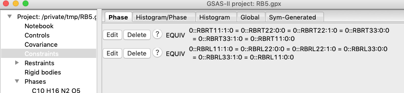
7D) Create constraints on the L_jj terms through use of the Constraints tree item as was done before. Their variable name is RBRLjj:b:0. Again use the “Edit Constr.”/“Add Equivalence” menu item and enter RBRL in the search filter. The first term is one of the six that needs to be constrained, and on the next screen select the remaining five 11, 22 and 33 terms and press OK. Constraints should appear as:

7E) Then refine with these parameters and the Rwp remains at 2.5%, but I would argue this is a more reasonable model than the Uiso model. If the thermal ellipsoids are plotted, they get larger further away from the origin as one might expect.

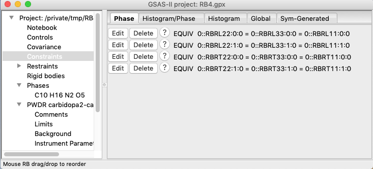
7F) An even more relaxed model would be to allow the T_jj and L_jj terms to differ between the two bodies, with constraints as shown below, but this produces no improvement in the Rwp. Further it has a non-physical negative L_jj value for one of the two bodies, so this is not a better model.

Conclusion

In this tutorial, we have seen how to create a rigid body, using the Avogadro program to regularize the internal geometry. The body was then imported into GSAS-II, including 4 torsion angles internal to the body. The rigid body was then placed into the unit cell in previously determined positions/orientations. The positions, orientations and torsions, as well as rigid body group motion parameters, were then refined. The resulting fit was excellent, with a highly realistic structure and a small number of parameters that are appropriate for the dataset being used.