RMCProfile – IV
Introduction
In this
tutorial, we will show how to use GSAS-II in conjunction with RMCProfile
(“RMCProfile: Reverse Monte Carlo for polycrystalline materials”, M.G. Tucker,
D.A. Keen, M.T. Dove, A.L. Goodwin and Q. Hui, (2007) Jour. Phys.: Cond.
Matter, 19, 335218. doi: https://doi.org/10.1088/0953-8984/19/33/335218)
to do a fit with x-ray powder diffraction data and pair distribution functions
(PDF) created from it with a “big box” disordered model. This exercise is very
similar to RMCProfile-III except that no neutron data is used and instead a set
of bond and angle potentials are used to augment the fitting.
Before
getting started you must obtain the most recent Version 6 of the RMCProfile
executable (at this writing this is RMCProfile V6.7.9 although V6.7.6 will also
work, but not any earlier version). Obtain this from www.rmcprofile.org by following the
prompts from Downloads. This version is available for Windows, Mac OSX and
Linux. The download will be a zip file; save it somewhere convenient. Pull from
it only the RMCProfile_package/exe/rmcprofile.exe and the two files in RMCProfile_package/exe/cuda_lib
(if present) and place them in the GSASII main directory or in a new
subdirectory (e.g. GSASII/RMCProfile); no other files are needed although you may
wish to also retrieve the contents of the tutorial subdirectory. It contains rmcprofilemanual.pdf and rmcprofile_tutorial.pdf which may be of interest
since the GSAS-II/RMCProfile tutorials are based on the latter.
The
process for using RMCProfile begins with a normal Rietveld refinement of the
average structure. For the kind of disordered materials of interest here, this
may give bond lengths that are frequently too short for the atoms involved and
sometimes extreme apparent thermal motion for some of the atoms. These effects
arise because the average structure places these atoms too close to one
another; a more localized view would show coordinated atom displacements or
reorientation of groups of atoms to avoid the close contacts. RMCProfile is
then used to characterize these local displacements by fitting to the
diffraction data and its Fourier transform as a PDF.
The
material used in this tutorial is the same as described in the RMCProfile-III
tutorial, gallium phosphate (GaPO4). GaPO4 is a
piezoelectric crystal of corner sharing GaO4 and PO4
tetrahedra arranged as in a doubled c-axis α-quartz structure. The average structure determined by Rietveld
refinement results in Ga-O and P-O bond lengths that are shorter than implied
by the corresponding peak positions in either an x-ray or neutron PDF. The
X-ray data used here was obtained at room temperature on beam line I15 at the
Diamond light source. The objective here is to use RMCProfile to model the
structural distortions that yield the X-ray PDF derived bond lengths and is
augmented by potential energy restraints on Ga-O and P-O bond lengths and
O-Ga-O and O-P-O bond angles. The result obtained here can be compared to that
from the combined x-ray/neutron fitting described in the RMCProfile-III
tutorial.
If you have not done so already, start GSAS-II.
Rietveld Refinement of Gallium phosphate (GaPO4):
Step 1: Read in the data file
1. Use
the Import/Powder Data/from GSAS powder data file menu item
to read the data file into the current GSAS-II project. This read option is set
to read any of the powder data formats defined for GSAS (angles in centidegrees, TOF in µsec). Other submenu items will read
the cif
format or the xye
format (angles in degrees) used by topas, etc. In those cases, you would change the file
type to cif
format or the xye
format (angles in degrees) to see them. Because you used the Help/Download tutorial
menu entry to open this page and downloaded the exercise files (recommended),
then the RMCProfile-IV/data/...
entry will bring you to the location where the files have been downloaded. (It
is also possible to download them manually from https://advancedphotonsource.github.io/GSAS-II-tutorials/RMCProfile-IV/data/.
In this case you will need to navigate to the download location manually.)
For this tutorial you should see the data file in the file
browser, but if extensions on data files are not the expected ones, you may
need to change the file type to All files (*.*) to
find the desired file.
2. Select the 105870-pe-GaPO4_ed.gsas data
file in the first dialog and press Open.
There will be a dialog box asking Is this the
file you want? Press Yes
button to proceed.
Next
will be a apparently empty file selection dialog for the instrument parameter
file; switch the file type to GSAS iparm file (*.prm,…). Then one file (inst_i15_pdf_april14.prm) is shown. Select it; the
pattern will be read in and displayed
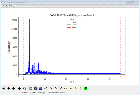
Step 2. Set limits
Since
we want to avoid the abrupt jump and (as it turns out) low angle contaminating
peaks, we want to set the lower limit to just below the first large visible
Bragg peak and the upper limit needs to be set to include just the range with
Bragg intensities (>0.4Å); go the Limits entry in the GSAS-II data
tree.
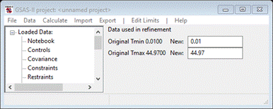
Change
the 1st entry to 2 and the second to 25; the plot will change by moving the green and red dashed
lines.

Step 3. Import GaPO4
phase
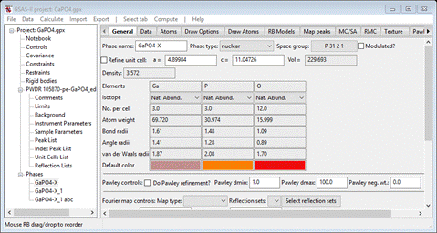
The average structure of GaPO4 is that of a doubled c-axis α-quartz. Space group P3121, a=4.90063 c=11.04809 with 4 atom positions. We can import it from an old gsas experiment file. Use the Import/Phase/from GSAS .EXP file menu item to read the phase information for GaPO4 into the current GSAS-II project. Other submenu items will read phase information in other formats. Because you used the Help/Download tutorial menu entry to open this page and downloaded the exercise files (recommended), then the RMCProfile-IV/data/... entry will bring you to the location where the files have been downloaded. (It is also possible to download them manually from https://advancedphotonsource.github.io/GSAS-II-tutorials/RMCProfile-IV/data/. In this case you will need to navigate to the download location manually.) Select the GAPO4_XRAY_BAK.EXP file (only one there) There will be a dialog box asking Is this the file you want? Press Yes button to proceed. You will get the opportunity to change the phase name next (it is very long, I changed it to GaPO4-X; this will be used as the file root for many of the files produced by RMCProfile. NB: because of restrictions in RMCProfile it is important that the phase name not have any spaces); press OK to continue. Next is the histogram selection window; this connects the phase to the data so it can be used in subsequent calculations.

Select the histogram (or press Set All) and press OK. The General tab for the phase is shown next
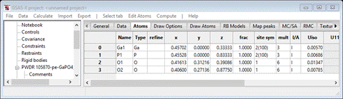
Step 4. Check atom
positions
It
is usually wise particularly for trigonal/hexagonal structures, to check the
atom positions to be sure atoms are properly placed on special positions. Select
the Atoms tab
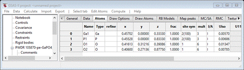
In
this case the z-position for both Ga and P are not sufficiently precise for use
in RMCProfie. The Ga atom is at z=1/3 and the P atom is at z=5/6. Enter the fractions into
the respective positions in the table; GSAS-II will do the math to the full
double precision available in python. You should get
If
this isn’t done then some of the input to RMCProfile will not be correctly
prepared.
Step 5. Set the
background
Although
there is not much diffuse scattering, the default background will be
insufficient for reasonable fitting. Select the Background item from the GSAS-II data
tree
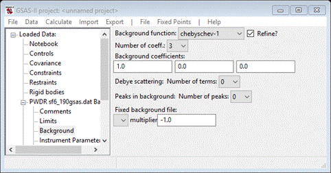
Be
sure that “chebyschev-1” is used for the background function; RMCProfile only
recognizes that form to compute the background for the diffraction pattern.
Select 6 for the number of terms.
Step 6. Rietveld
refinement
We
are now ready for the first Rietveld refinement; select Calculate/Refine from the main GSAS-II menu.
Before it starts a file selection dialog will appear; select a file name (no
extension). I chose “GaPO4”; do not use the phase name for this purpose because
RMCProfile will use that as the root for the many files it creates. Also, you
should create a new directory for this exercise while in this dialog box; it
will be rapidly filled up with RMCProfile files which can lead to considerable
confusion if mixed in with other files. For Windows, after navigating to a
suitable location, a new directory can be made by a right mouse click and
selecting “New/Folder” from the popup menu. It will appear with the name “New
Folder”; change the name and select it (it will be empty). Other operating
systems will have similar methods. Finally press Save to save the GSAS-II project
(GaPO4.gpx) and start the refinement. It will quickly converge to give a
reasonable Rwp (~9.8%)
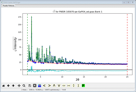
I
pressed the ‘s’ key so that sqrt(intensity) shows on the y-axis; makes things a
bit easier to see. It is evident that the lattice parameter as well as the
sample broadening terms needs adjusting. Go to the General tab for the GaPO4-X phase
and select Refine unit cell. Then select the Data tab and select size and microstrain for refinement. (A word to
the wise; set the starting value for size to 0.1 μm). Then do Calculate/Refine
from the
main menu. The fit will greatly improve (Rwp ~5.25%)

To
finish up add the following parameters:
GaPO4-X/Atoms: XU for all four atoms (GSAS-II
recognizes that the Ga & P atoms are fixed in y & z positions).
Do Calculate/Refine from the main menu; the fit
will scarcely change (Rwp~5.25%).
Step 7. Draw
structure
Select
the Phases/GaPO4-X/Draw
Atoms tab;
the list will be shown and the four unique atoms drawn on the plot.

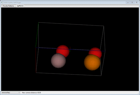
To
improve this do the following:
1)
Double click the empty upper left box in the Draw Atoms table; all atoms will turn
green and the four table rows will be grey (or blue).
2)
Under the menu Edit Figure select Fill unit cell; the figure will be redrawn
showing all atoms in the cell.
3)
Double click the Type column heading and select the Ga and P atom types
4)
Under the menu Edit Figure select Fill CN-sphere; the figure will be redrawn
with four O atoms about all Ga and P atoms.
Next we will explore this with a
RMCProfile simulation. To keep this drawing, you may want to save the GSAS-II
project.
Reverse Monte Carlo
Simulation of GaPO4
RMCProfile
is most effective if a large box is used for the modelling; this requires very
long running times (10-20 hrs for GaPO4)
before a meaningful result is obtained. However, for the purposes of this
tutorial, we will be using a smaller box model that converges in a more reasonable
time (~10min). The result will clearly fit the data but the model is too small
to give enough atom displacements to be meaningful, however this exercise will
show you how to set up RMCProfile from within GSAS-II.
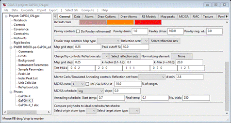
To
start select the Phases/GaPO4-X/RMC tab; if rmcprofile.exe is
within the GSASII directory the data window will show
At
the top is a radio button selection for RMCProfile and fullrmc. The latter is an
alternative big box modeling program (not working – under development);
RMCProfile is selected by default and all below are its setup controls. There
are four major sections (metadata, major controls, restraints & constraints
and data controls); we will work through each of these in turn. The information
you enter here is retained in the GSAS-II project file so you can easily try
alternative setups without having to enter everything over again.
Step 1. Set
metadata items
The
entries here are for your convenience; there is no explicit use made of any of
them, but they will appear in some of the output files from RMCProfile and of
course will show here on subsequent views of this window. Fill out as many of
them as you see fit. I entered some things for each as the defaults are
somewhat nonsensical.
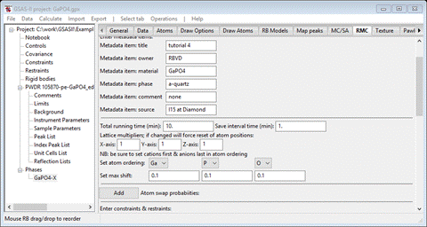
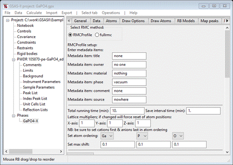
Step 2. Set general
controls
The
running time is defaulted to 10 minutes with a Save interval of 1 minute. At each save time a
number of files are written by RMCProfile; these can be viewed by using the
Operations/Plot command (more about this later – don’t bother trying it now,
there is nothing to see). For the purposes of this tutorial leave them at their
defaults.
The
big box model used by RMCProfile is described as multiples of the unit cell
axes. In this case we want a 6x6x4 box so enter 6 for each of X-axis, Y-axis and 4 for Z-axis.
Next
is to set the order of the atom types in the structure; this is used to
construct atom-atom distance restraints on the modelling. The order here (Ga, P, O) is appropriate; if changed
the window will repaint updating various entries possibly resetting some
entries to defaults. I suggest you decide the order now and then don’t change
it later. Set the maximum shift for Ga & P to be 0.05 (the value for O is OK).
When done the window should look like

Skip
the next item (Atom swap probabilities). This is for cases in which atoms can
exchange sites.
Step 3. Set
constraints/restraints
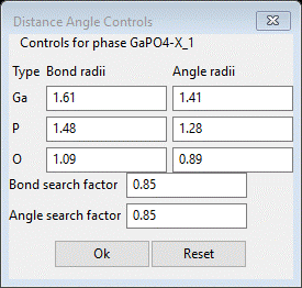
Next
is to set the “Hard” minimum atom-atom separation and the allowed search rage
for each of 6 pairs of atom types. Possible values for this table can be
obtained in GSAS-II by computing bond lengths although we discovered a good set
in the RMCProfile-III tutorial; we will use these here. Suitable values are in
sequence for Hard min and Search from: 4.0, 2.6, 1.2, 4.0, 1.2, 2.16.
The to items are: 4.8, 3.4, 2. 4.8, 2.0, 0.0. When done the window should
look like
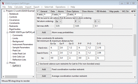
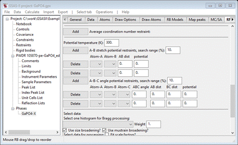
Scroll
down to find the section that has “Potential temperature”; these are for bond
and angle potentials. We will need 2 of each so press Add (twice) for A-B stretch and Add (again twice) for A-B-C
angle potentials; the window will refresh for each press so be patient while it
does this. Additional entries will be formed for each; when done the window
will look like
We’re
wanting Ga-O and P-O stretch potentials and O-Ga-O and O-P-O angle potentials. Select the
Atom-A, Atom-B and Atom-C appropriately to give
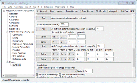
Next
enter appropriate Ga-O and P-O bond distances (1.81 and 1.51) and O-Ga-O and O-P-O angles
(the ideal tetrahedral angle 109.5) and set all potentials to 2.0. Set both search ranges to 20%. When done you should see

Step 4. Select data
to be fitted
We
will be using just x-ray data for GaPO4 for fitting by RMCProfile.
The first step is the selection of the x-ray powder pattern (“Bragg”) for
processing. This is taken from the PWDR entry in the GSAS-II project and
accessed from the pulldown; there is only one “PWDR 105870-pe-GaPO4_ed.gsas Bank
1” that was
used earlier in your Rietveld refinement of GaPO4. If you had used
multiple banks in the Rietveld refinement, all would be shown in the pulldown,
but only one can be selected. Set the weight to 100 (NB: smaller numbers means a
heavier weight).
Next
press the Select button for the “Xray reciprocal space data: F(Q)” line; a FileDialog
should appear. Because you used the Help/Download tutorial
menu entry to open this page and downloaded the exercise files (recommended),
then the RMCProfile-IV/data/...
entry will bring you to the location where the files have been downloaded. (It
is also possible to download them manually from https://advancedphotonsource.github.io/GSAS-II-tutorials/RMCProfile-IV/data/.
In this case you will need to navigate to the download location manually.)
The FileDialog should show

Select
gapo4_xray_rmc.fq; it will be copied to your
working directory. The window will be redrawn; set the weight to 0.1. You should also check the Fit scale
factors?
box. When done the window should show
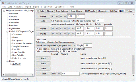
You
should do a Save project here.
Step 5. Setup
RMCProfile files
You
are now ready to setup the RMCProfile input files. Do Operations/Setup
RMC from the
menu; the console should report that files were written

and
your local directory should now have at least these 9 files

These
text files contain data needed by RMCProfile for the fitting of GaPO4.
They are:
GaPO4-X.back- the 6 coefficients for the
chebyschev-1 function needed to compute the background for the Bragg pattern
GaPO4-X.bragg – the powder pattern used in
the Rietveld refinement
GaPO4-X.dat – the RMCProfile controls
file; described in full in the RMCProfile User Manual. It can be edited if need
be, but remember it is rewritten each time Operations/Setup RMC is done.
GaPO4-X.inst – the instrument parameter
coefficients for the x-ray peak shape function used by GSAS-II and implemented
in RMCProfile for computing the Bragg pattern.
GaPO4-X.rmc6f – the big box set of atom positions.
It is normally not rewritten when Operations/Setup RMC is done unless the
X-axis, Y-axis, or Z-axis lattice multipliers are changed. Most important is
that it will contain the set of big box atom positions as updated by RMCProfile
according to the Save interval (every 1 min in this case).
You
are now ready to run RMCProfile.
Step 6. Run
RMCProfile
To
run RMCProfile from inside GSAS-II, do Operations/Execute. You will first see a “nag”
note asking you to cite the publication describing RMCProfile; press OK. The program will start in a
new console window – processing will initially be pretty fast for this case and
then slow down as the modelling proceeds. It reports Time used and Last saved.
Once the latter is nonzero you can view intermediate results to see its
progress.

I
have captured the initial RMCProfile console output (done by simply clicking
anywhere in the window – note the white square. This temporarily stops processing;
it can be restarted by pressing any key with the focus on the window). Things
to look at are the several chi^2 values; there will be an overall one and one
for each of the 3 data sets used in the fitting. The last one “X-ray
real-space” is generated within RMCProfile by doing the Fourier transform from
the F(Q) input data to form the x-ray g(R) distribution (e.g. the x-ray PDF).
Since we’ve set the Fit scale factors option; the “Renorm”
values are other than unity. These will approach 1.0 as the modelling
continues. There is also a value for Bond energy calculated from the bonds and
angles subject to the potential energy restraints. Do not be surprised if this
value rises while RMCProfile runs; that is simply a reflection of the
distortions found in this structure. It will peak at about the 4-5 min mark and
then decrease after that. Note that you can exit GSAS-II and RMCProfile will
continue running. When it finished the console shows (in part)
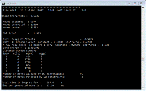
The
chi^2 values are now close to unity and not very different from each other;
this is what is desired. The bond energy started out at ~8700, peaked at
~14,000 and now is ~11,500; this is the effect of the distortions found by
RMCProfile.
After
RMCProfile finishes note that the project directory now has ~35 files many of
which are just temporary ones created by RMCProfile. We will be looking at just
the *.csv files and the GaPO4.rmcf6 file; the latter contains the last atom
configuration acceptable by RMCProfile thus representing a best disordered
model.
A note about
weights:
The
choice of weights for RMCProfile may seem to be arbitrary in these exercises, but
I have selected them so that each of the chi^2 values converge to be roughly
equal and somewhere near unity. This selection generally gives the best
performance in the reverse Monte Carlo calculation and requires some “trial
& effort” in selecting the values. If one of the chi^2 values is too large
(>>1, i.e. weight too small) at convergence, then adjustments in the
structure will have been dominated by moves that lower that chi^2 sometimes at
the expense of others. Conversely, if one chi^2 is too small (>>1, i.e.
weight too large) then moves will tend to satisfy the others and there will be
little sensitivity to that data set. In this case my chosen weights have
yielded chi^2 values between 0.5 and 2.0; this is essentially ideal. If they
vary by more than an order of magnitude or are much greater or less than unity,
you should adjust the weights.
Step 7. Viewing
results from RMCProfile
Do Operations/Plot; a FileDialog
showing only *.csv files will appear

They
all should have the same prefix in their name, “GaPO4-X” which is the phase
name from the GSAS-II project file. Select any one of them – it doesn’t matter.
All of them will be read and their contents displayed as individual plots. For
example the chi^2 plot shows the progress of the RMCProfile fit
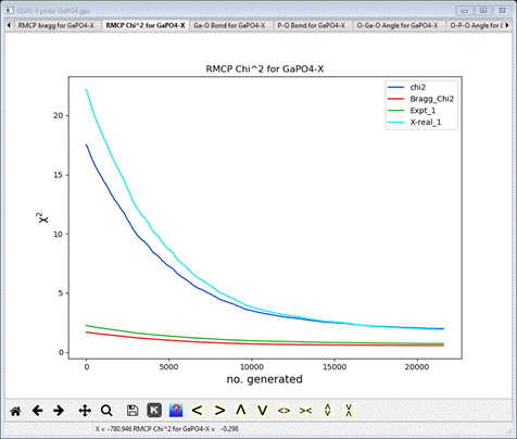
If
you zoom into the end of the run, you can see that RMCProfile is still
improving the fit slowly even after 10 minutes of running.
Comparing the Bragg plot with the PWDR plot shows that the
RMCProfile fit is very similar to the Rietveld fit
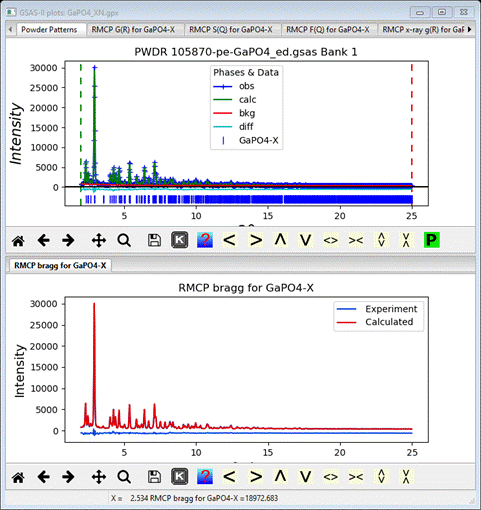
This
plot was made by dragging one plot tab to the bottom of the screen to create
the second frame.
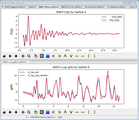
A
consideration of the reciprocal space F(Q) (top) and the x-ray real space g(R)
(bottom) plots show reasonable agreement between the RMCProfile model and the
data (but not quite as good as we obtained in the RMCProfile-III tutorial –
probably an effect of imposing the potential energy restraints.
The
bonds and angles subject to potential energy restraints are plotted
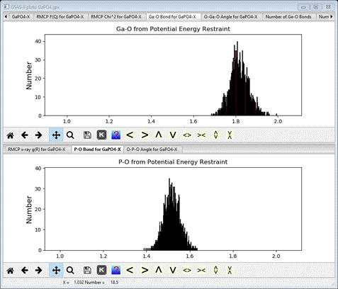
I’ve
adjusted the scales to give a better view of the different bond lengths.
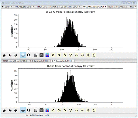
On
the other hand, the bond angles are essentially the same as the ideal
tetrahedral angle but with considerable spread (close to +/- 10 deg).
Finally,
note that the console gave mean values for the bonds and angles that were
restrained by potential energy functions.
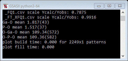
These
agree pretty well with our supposed values entered for these restraints. If our
guesses were wrong then there would be a shift; one can then enter the new
values, redo Operations/Setup RMC and then repeat Operation/Execute to rerun
RMCProfile which would start where the previous run stopped.
Step 9. View the
big box structural model for GaPO4
Next,
we can view the resulting big box structure. Do Import/Phase/from RMCProfile
.rmc6f file;
a FileDialog box with one entry will show the
required file, GaPO4-X.rmc6f. You will first see a Is this the
file you want
popup window; select Yes. Next will be an Edit phase name popup. The proposed name is
the same as the existing one; GSAS-II will rename this one by adding ‘_1’ to
the end. Next will be a popup for Add histograms; respond Cancel because you don’t want this
phase to be in any subsequent Rietveld refinement. Looking at the General tab for this phase we see it is 6X in a & b and 4X in c
axes relative to the original and has no symmetry (space group P 1).

Select
the Draw
Atoms tab
for this phase; a van der Waals ball model will be drawn. You can select the Ga & P atoms & fill the CN-sphere for them (does take a long
time, >10min – be patient) and then change all the atoms to ball and stick
style. The CN-sphere filling works because the RMCProfile structure still has
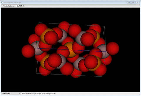
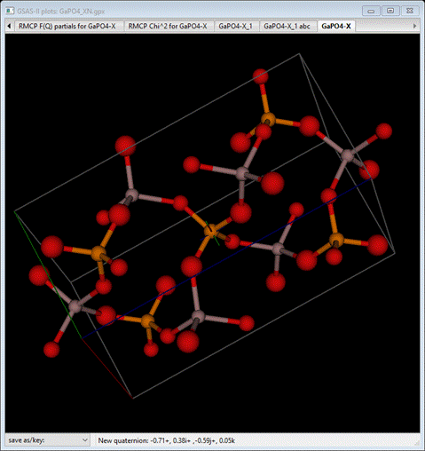
translational symmetry across its 6x6x4 lattice. You should see something like
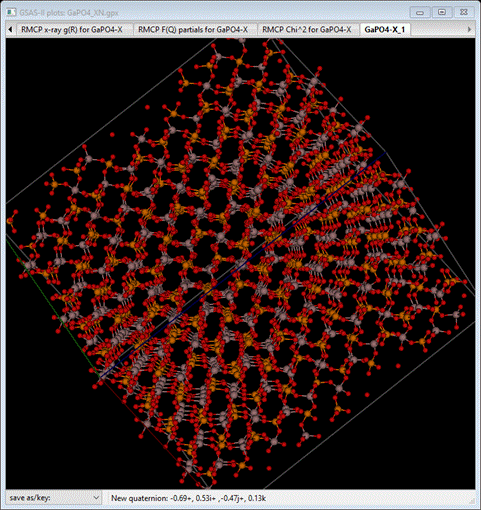
Notice
the apparent tilting the PO4 and GaO4 tetrahedra. The stray
O atoms are bound to PO4 and GaO4 tetrahedra in
neighboring boxes.
NB:
this import facility can be used to load any rmc6f file, e.g. from a RMCProfile
run done outside of GSAS-II; all the plotting and tools in this and the
following steps are available for these big box models.
Step 10. View the
disordered average structure
We
can compress the big box result back into the original average crystal structure
to see how the disordered sites compare with the average ones. Select the General tab for the big box phase
(SF6_1) and then do Compute/Transform. A popup dialog will appear

This
is the general tool inside GSAS-II for all sorts of structure transformations.
Here we will use it to push all the big box atoms back into the average
structure unit cell. Recalling that the big box model is 6x6x4 the original
unit cell, we simply want to reverse the process. Enter 1/6, 1/6,1/4 into the diagonal elements
of the M matrix. The GUI will convert them to the decimal equivalent (0.167,…). The target space group should be P 1. You should
see

Press
Ok to do the transformation. A
new phase, “GaPO4-X_1 abc” will be formed as
triclinic with cell axes that match the original hexagonal ones. Select Draw Atoms; a van der Waals model will
appear.

Select
the Draw
Options tab
and reduce the van der Waals scale to about 0.05.
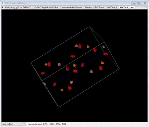
This
compares pretty well with the original structure with the ellipsoids drawn at
99% probability. If anything the spread in atom positions is less that what was
obtained in the RMCProfile-III tutorial; an effect of the potential energy
restraints.
However,
the O atoms are more widely distributed in space than the P or Ga atoms.
Step 11. Polyhedral
comparison for the big box model
In
this step we will examine how the suite of PO4 and GaO4
tetrahedra deviate from an ideal tetrahedron. This analysis is currently
restricted to structures with P1 space group symmetry; this is what we have
from Step 9 above. Select Phases/GaPO4-X_1 from the data tree; the
General tab will appear.

What
we want is at the bottom of this panel; scroll down to the bottom
At
the very bottom is the control for polyhedral comparison. All that is needed is
to select the central atom (“origin atom type”) and the polyhedral
vertices (“target atom type”). Select P for the former and O for the latter. Then do Compute/Compare from the menu; a popup for
setting Distance Angle Controls will appear
In
some cases the bond search factor may need to be adjusted to get the right
number of vertices for the polyhedra; in this case 0.85 is fine (NB: in this use the
angle ranges are ignored). Press OK; a progress bar will show the atoms being processed. The
console may show some atoms being skipped because the number of vertices wasn’t
either 4 (tetrahedron) or 6 (octahedron); all but one are ok here. Because
there are 432 P atoms to be looked at in this big box model, this calculation
can take a number of minutes. The General tab reappears already scrolled to the
bottom
A
new button (Show Plots?) has appeared after the atom selections; press it. A number
of new entries will appear on the plot window; we will discuss each in turn.
Select the Tet P-O Bond for GaPO4-X_1 tab
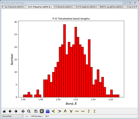
This
gives the distribution of the average P-O bond lengths for all the tetrahedra
found across the big box model. It is rough because of the small size of the
model, but the asymmetry seen in the RMCProfile-III is not present in this P-O
bond distribution. The console will have listed the average value with the
standard uncertainty in parentheses.

Next
select the Tet P-O Tilts for GaPO4-X_1tab
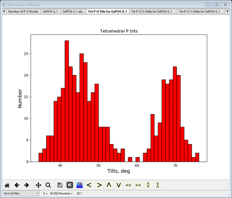
This gives the distribution of axial tilts of the PO4
molecules from the reference tetrahedron (aligned along the Cartesian axes) and
is similar but tighter compared to that found in the RMCProfile-III tutorial.
There is an apparent split distribution centered at ~48 deg and ~68 deg (the
rather meaningless in this case average tilt is also shown on the console).
Next select X-Delta, Y-Delta and Z-Delta tabs in turn.
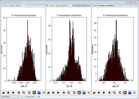
I
have made this plot by dragging the respective plot tabs to one of the right
(or left) edges to create a 3 pane plot. These show the displacement of the O
atoms from the ideal tetrahedral vertices along each Cartesian axis. Here they
are arranged about the zeros fairly tightly; the apparent split in the DY plot may or may not be
real. If there were structural distortions to the tetrahedra (e.g. Jahn-Teller
distortions) these could show in these plots.
To
do the same thing for Ga-O polyhedra, select Ga instead of P for the origin type atom and then do Compute/Compare. Again there will be the Distance Angle Controls popup; no changes needed.
The calculation will again take several minutes to complete. When done press
the Show plots? button; more plots will be
added to the plot window. I show both sets of tetrahedral bonds as a stacked
plot; the Ga-O bonds are not skewed, either. 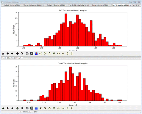
Similar
comparisons can be made with the other plots. NB: if the project is now saved
all the data needed to reproduce the plots is also saved; any of them can be
seen without redoing the Compare calculation.
This
completes this RMCProfile tutorial; you should save the project.
Final note
A
production run with enough atoms to give decent statistics would be for a box
that is perhaps 12x12x8 the original unit cell and would require a 10-20 hour
run time. It would contain several thousand atoms instead of ~2600 as used
here. You can further explore this tutorial project by changing the bond and
angle potentials to see how that changes the RMCProfile result. In my case,
increasing all 4 to 20 from 2 tightened the Ga-O and P-O bond length
distributions but had no impact on the O-P-O and O-Ga-O angle distributions.
The fit to the g(R) is also poorer (much higher chi^2).