RMCProfile – II

· Exercise files are found here

Introduction

In this tutorial, we will show how to use GSAS-II in conjunction with RMCProfile (“RMCProfile: Reverse Monte Carlo for polycrystalline materials”, M.G. Tucker, D.A. Keen, M.T. Dove, A.L. Goodwin and Q. Hui, (2007) Jour. Phys.: Cond. Matter, 19, 335218. doi: https://doi.org/10.1088/0953-8984/19/33/335218) to fit both neutron powder diffraction data and a pair distribution function (PDF) created from it with a “big box” disordered model.

Before getting started you must have the most recent Version 6 of the RMCProfile executable (at this writing this is RMCProfile V6.7.9 although V6.7.6 will also work, but not any earlier version). Obtain this from www.rmcprofile.org by following the prompts from Downloads. This version is available for Windows, Mac OSX and Linux. The download will be a zip file; save it somewhere convenient. Pull from it only the RMCProfile_package/exe/rmcprofile.exe and the two files in RMCProfile_package/exe/cuda_lib (if present) and place them in the GSASII main directory or in a new subdirectory (e.g. GSASII/RMCProfile); no other files are needed although you may wish to also retrieve the contents of the tutorial subdirectory. It contains rmcprofilemanual.pdf and rmcprofile_tutorial.pdf which may be of interest since the GSAS-II/RMCProfile tutorials are based on the latter.

The process for using RMCProfile begins with a normal Rietveld refinement of the average structure. For the kind of disordered materials of interest here, this may give bond lengths that are frequently too short for the atoms involved and sometimes extreme apparent thermal motion for some of the atoms. These effects arise because the average structure places these atoms too close to one another; a more localized view would show coordinated atom displacements or reorientation of groups of atoms to avoid the close contacts. RMCProfile is then used to characterize these local displacements by fitting to the diffraction data and its Fourier transform as a PDF.

The material used in this tutorial is the same as described in the RMCProfile tutorial Exercise 4, strontium titanate (SrTiO₃). In this perovskite the TiO6 octahedra are slightly tilted to accommodate the Ti-O bond length in a slightly too small unit cell. The data used here was obtained at 190K on the GEM diffractometer at ISIS, Rutherford-Appleton Laboratory, Harwell Campus, UK. The process of creating this data introduced two minor flaws: one is a slight mis-scaling of the magnitudes of the real space, G(R), and reciprocal space, F(Q), patterns and the other is a difference in the diffractometer constant, difC, used to make them vs that used for the Rietveld refinement. In this tutorial we will address both of these in case you encounter them in your future work with RMCProfile.

If you have not done so already, start GSAS-II.

Rietveld Refinement of Strontium titanate (SrTiO₃):

Step 1: Read in the data file

1. Use the Import/Powder Data/from GSAS powder data file menu item to read the data file into the current GSAS-II project. This read option is set to read any of the powder data formats defined for GSAS (angles in centidegrees, TOF in µsec). Other submenu items will read the cif format or the xye format (angles in degrees) used by topas, etc. In those cases, you would change the file type to cif format or the xye format to see them. Because you used the Help/Download tutorial menu entry to open this page and downloaded the exercise files (recommended), then the RMCProfile-II/data/... entry will bring you to the location where the files have been downloaded. (It is also possible to download them manually from https://subversion.xray.aps.anl.gov/pyGSAS/Tutorials/RMCProfile-II/data/. In this case you will need to navigate to the download location manually.)

For this tutorial you should see the data file in the file browser, but if extensions on data files are not the expected ones, you may need to change the file type to All files (*.*) to find the desired file.

2. Select the gem05984.gss data file in the first dialog and press Open. There will be a Dialog box asking Is this the file you want? Press Yes button to proceed. The data file contain 4 banks of data

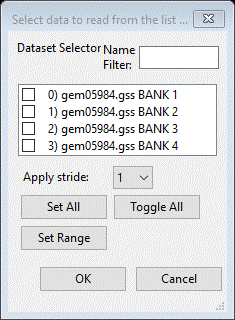
Select only the third one (BANK 3) and press OK. Next will be a file selection dialog for the instrument parameter file; only one (GEM.instprm) is shown. Select it; the pattern will be read in and displayed

This is a nice pattern showing very little evidence of disorder except that the three largest peaks appear to have satellite reflections on either side of the main peak so it is possible that an alternative to what we will be doing here is to describe the structure as incommensurate with some modulation of the anticipated small rotations of the TiO₆ octahedra.

Step 2. Set limits

The default limits are set in GSAS-II to be something typical starting at 0.4Å; there is useful data over the entire range starting at 0.33Å, so let’s use it all.

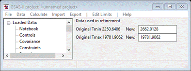
On the plot drag the green dashed line to the left beyond the data; it will snap to the lowest limit of the data and update the limits table. The upper limit is fine.

Step 3. Import SrTiO₃ phase

The average structure of SrTiO₃ is very simple. Space group I4/mcm, (or Im-3m; a=5.48, c=7.75 with Ti at 0,0,0, Sr at ½,0,¼ and O at 0,0,¼ and .241,.258,0. However, we will save time by importing it from an old gsas experiment file which has anisotropic thermal motion for the O atoms. Use the Import/Phase/from GSAS .EXP file menu item to read the phase information for SrTiO₃ into the current GSAS-II project. Other submenu items will read phase information in other formats. Because you used the Help/Download tutorial menu entry to open this page and downloaded the exercise files (recommended), then the RMCProfile-II/data/... entry will bring you to the location where the files have been downloaded. (It is also possible to download them manually from https://subversion.xray.aps.anl.gov/pyGSAS/Tutorials/RMCProfile-II/data/. In this case you will need to navigate to the download location manually.) Select the SRTIO3_5K.EXP file (only one there) There will be a Dialog box asking Is this the file you want? Press Yes button to proceed. You will get the opportunity to change the phase name next (change it to ‘SrTiO3’; NB: because of restrictions in RMCProfile it is important that the phase name not have any spaces); press OK to continue. Next is the histogram selection window; this connects the phase to the data so it can be used in subsequent calculations.

Select the histogram (or press Set All) and press OK. The General tab for the phase is shown next

Step 4. Set the background

Select the Background item from the GSAS-II data tree

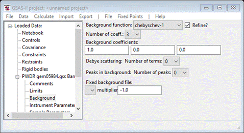
Be sure that “chebyschev-1” is used for the background function; RMCProfile only recognizes that form to compute the background for the diffraction pattern. Select 6 for the number of terms.

Step 5. Rietveld refinement

We are now ready for the first Rietveld refinement; select Calculate/Refine from the main GSAS-II menu. Before it starts a file selection dialog will appear; select a file name (no extension). I chose “SrTiO3_5K”; do not use the phase name for this purpose because RMCProfile will use that as the root for the many files it creates. Also, you should create a new directory for this exercise while in this dialog box; it will be rapidly filled up with RMCProfile files which can lead to considerable confusion if mixed in with other files. For Windows, after navigating to a suitable location, a new directory can be made by a right mouse click and selecting “New/Folder” from the popup menu. It will appear with the name “New Folder”; change the name and select it (it will be empty). Other operating systems will have similar methods. Finally press OK to save the GSAS-II project (SrTiO3_5K.gpx) and start the refinement. It will quickly converge to give a poor Rwp (~44%) mostly because of mismatches in peak positions

It is evident that the lattice parameter needs adjusting. Go to the General tab for the SrTiO₃ phase and select Refine unit cell; repeat Calculate/Refine. The Rwp will improve (~15.9%) giving

To finish up add the following parameters:

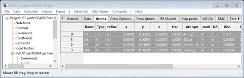
SrTiO3/Atoms: XU for all four atoms (GSAS-II recognizes that some are fixed in position); the O atoms should have anisotropic thermal displacements.

SrTiO3/Data: refine microstrain and leave size at 1.0.

PWDR/Instrument Parameters: refine difA, Zero, beta-0, beta-1, sig-0, sig-1 and sig-2 (normally not necessary, but the available GEM instrument parameter file isn’t current). In any event, the coefficients difB, beta-q and sig-q must be zero since RMCProfile V6.7.6 Beta Serial does not know how to use them in computing a powder profile.

Do Calculate/Refine from the main menu; the fit will improve some more to Rwp ~ 7.24% (you may have to repeat Calculate/Refine to get to convergence)

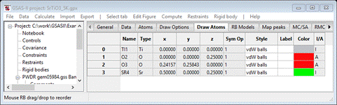
Step 6. Draw structure

Select the Phases/ SrTiO3/Draw Atoms tab; the list will be shown and the four unique atoms drawn on the plot.

To improve this do the following:

1) Double click the Style column heading and select ellipsoids; the figure will be redrawn showing the 50% ellipsoid surfaces (very small!)

2) Double click the empty upper left box in the Draw Atoms table; both atoms will turn green and the four table rows will be grey.

3) Under the menu Edit Figure select Fill unit cell; the figure will be redrawn showing all atoms in the cell (too many bonds, though).

4) Double click the Type column heading and select the Ti atom type

5) Under the menu Edit Figure select Fill CN-sphere; the figure will be redrawn with six O atoms about all Ti atoms (still too many bonds).

6) Finally select Draw Options tab, set the Ellipsoid probability all the way to the left (99%) and change Bond search factor to 0.8; the figure will be redrawn to show

which is what one expects for some kind of orientational disorder for the TiO₆ octahedra. If you look carefully you can see the slight twisting about the c-axis (that gives the tetragonal perovskite structure), but there is some additional tilting as well that leads to a disk-like shape to the axial O-atoms compared to the others. Next we will explore this with a RMCProfile simulation. To keep this drawing, you may want to save the GSAS-II project.

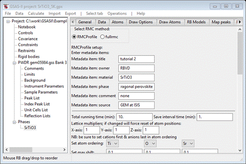
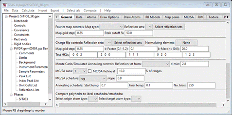
Reverse Monte Carlo Simulation of SrTiO₃

To start select the Phases/SrTiO3/RMC tab; if rmcprofile.exe is within the GSASII directory the data window will show

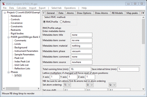
At the top is a radio button selection for RMCProfile and fullrmc. The latter is an alternative big box modeling program (not working – under development); RMCProfile is selected by default and all below are its setup controls. There are four major sections (metadata, major controls, restraints & constraints and data controls); we will work through each of these in turn. The information you enter here is retained in the GSAS-II project so you can easily try alternative setups without having to enter everything over again.

Step 1. Set metadata items

The entries here are for your convenience; there is no explicit use made of any of these, but they will appear in some of the output files from RMCProfile and of course will show here on subsequent views of this window. Fill out as many of them as you see fit. I entered some things for each as the defaults are somewhat nonsensical.

Step 2. Set general controls

The running time is defaulted to 10 minutes with a Save interval of 1 minute. At each save time a number of files are written by RMCProfile; these can be viewed by using the Operations/View command (more about this later – don’t bother trying it now, there is nothing to see). For the purposes of this tutorial leave them at their defaults.

The big box model used by RMCProfile is described as multiples of the unit cell axes. In this case we want a 6x6x4 box so enter 6 for each of X-axis, Y-axis and 4 for Z-axis.

Next is to set the order of the atom types in the structure; this is used to construct atom-atom distance restraints on the modelling. The order here (Ti followed by O and then Sr) isn’t appropriate; if changed the window will repaint updating various entries possibly resetting some entries to defaults. I suggest you decide the order now and then don’t change it later. Change it to Sr, Ti, O; the window will repaint each time. Set the maximum shift for Sr and Ti to be 0.05 (the value for O is OK). When done the window should look like

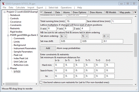
Skip the next item (Atom swap probabilities). This is for cases in which atoms can exchange sites.

Step 3. Set constraints/restraints

Next is to set the “Hard” minimum atom-atom separation and the allowed search rage for each of 6 pairs of atom types. Possible values for this table can be obtained in GSAS-II by computing bond lengths. Select the Atoms tab and then select all atoms by double clicking on the empty upper left box in the table.

Then do Compute/Show distances & angles from the menu; a popup will appear

Set the Bond search factor to 1.5 and the Angle search factor to 0.0 (to skip angle calculations), and press Ok. The console will show a very long table showing all interatomic distances out to 4-7Å. Find the shortest distance for each of the 6 types of atom pairs in the SrTiO3/RMC data tab. For each one subtract 0.2A and enter the value as Hard min and Search from. Then add 0.2A and enter that in the to row. When done the window should look like

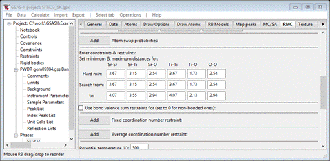
Scroll down to the bottom of the window for the last section.

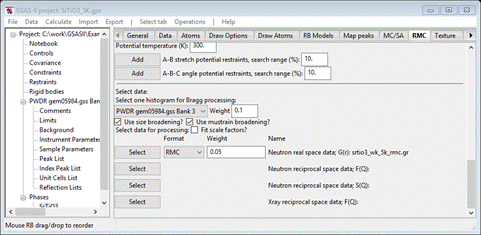
Step 4. Select data to be fitted

We will be using three different types of SrTiO₃ data for the fitting by RMCProfile. The first is the selection of the powder pattern (“Bragg”) for processing. This is taken from the PWDR entries in the GSAS-II project and accessed from the pulldown; there is only one “PWDR gem05984.gss Bank 3” that was used earlier in your Rietveld refinement of SrTiO₃. If you had used multiple banks in the Rietveld refinement, all would be shown in the pulldown, but only one can be selected. Set the weight to 0.5 (NB: smaller numbers means a heavier weight).

Next press the Select button for the “Neutron real space data; G(R)” line; a FileDialog should appear. Because you used the Help/Download tutorial menu entry to open this page and downloaded the exercise files (recommended), then the RMCProfile-II/data/... entry will bring you to the location where the files have been downloaded. (It is also possible to download them manually from https://subversion.xray.aps.anl.gov/pyGSAS/Tutorials/RMCProfile-II/data/. In this case you will need to navigate to the download location manually.)

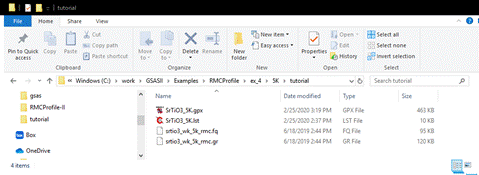
The FileDialog should show

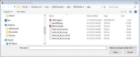
Select srtio3_wk_5k_rmc.gr; it will be copied from this location to your working directory for this tutorial (RMCProfile requires all its files to be local). The window will be redrawn showing the new entry; the weight is fine.

Next press the Select button for “Neutron reciprocal space data: F(Q)”; the FileDialog will show

Select srtio3_wk_5k_rmc.fq; again it will be copied to your working directory. The window will be redrawn

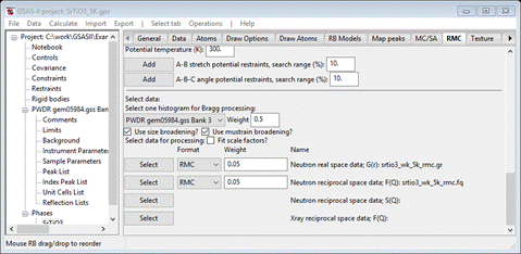
Again, leave the weight as it is. Your local directory should have just 3 or 4 files

Step 5. Setup RMCProfile files

You are now ready to setup the RMCProfile input files.. Do Operations/Setup RMC from the menu; the console should report that files were written

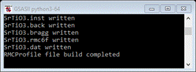
and your local directory should now have ~8 files

These text files contain data needed by RMCProfile for the fitting of SF6. They are:

SrTiO3.back- the 6 coefficients for the chebyschev-1 function needed to compute the background for the Bragg pattern

SrTiO3.bragg – the powder pattern used in the Rietveld refinement

SrTiO3.dat – the RMCProfile controls file; described in full in the RMCProfile User Manual. It can be edited if need be, but remember it is rewritten each time Operations/Setup RMC is done.

SrTiO3.inst – the instrument parameter coefficients for the neutron TOF peak shape function used by GSAS-II and implemented in RMCProfile for computing the Bragg pattern.

SrTiO3.rmc6f – the big box set of atom positions. It is normally not rewritten when Operations/Setup RMC is done unless the X-axis, Y-axis, or Z-axis lattice multipliers are changed. Most important is that it will contain the set of big box atom positions as updated by RMCProfile according to the Save interval (every 1 min in this case).

You are now ready to run RMCProfile.

Step 6. Run RMCProfile

To run RMCProfile from inside GSAS-II, do Operations/Execute. You will first see a “nag” note asking you to cite the publication describing RMCProfile; press OK.

The program will start in a new console window – processing will initially be fast for this case and then slow down as the modelling proceeds. It reports Time used and Last saved. Once the latter is nonzero you can view intermediate results to see its progress. It also shows the chi^2 for each of the contributing data sets; these start in the 5-300 range and will quickly drop in the initial stages of the run. Note that you can exit GSAS-II and RMCProfile will continue running. After RMCProfile finishes note that the project directory now has ~30 files many of which are just temporary ones created by RMCProfile. We will be looking at just the *.csv files and the SrTiO3.rmcf6 file; the latter contains the last atom configuration acceptable by RMCProfile thus representing a best disordered model.

A note about weights:

The choice of weights for RMCProfile may seem to be arbitrary in these exercises, but I have selected them so that each of the chi^2 values converge to be roughly equal and somewhere just above unity. This selection generally gives the best performance in the reverse Monte Carlo calculation and requires some “trial & effort” in selecting the values. If one of the chi^2 values is too large (>>1, i.e. weight too small) at convergence, then adjustments in the structure will have been dominated by moves that lower that chi^2 sometimes at the expense of others. Conversely, if one chi^2 is too small (>>1, i.e. weight too large) then moves will tend to satisfy the others and there will be little sensitivity to that data set. In this case my chosen weights have yielded 1.003 for the Bragg, 2.980 for the G(R) “Expt 1” and 1.899 for the F(Q) “Expt 2” data sets; this is essentially ideal. If they vary by more than an order of magnitude or are less than unity, you should adjust the weights.

Step 7. Viewing results from RMCProfile

Do Operations/View (you can do this any time after a save has been done); a FileDialog showing only *.csv files will appear

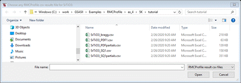
They all should have the same prefix in their name, “SrTiO3” which is the phase name from the GSAS-II project file. Select any one of them – it doesn’t matter. All of them will be read and their contents displayed as individual plots. For example the chi^2 plot shows the progress of the RMCProfile fit

The inset is the upper 3/4ths of the plot magnified; you can see that RMCProfile is still improving the fit slowly even after 10 minutes of running.

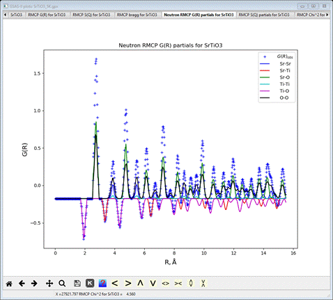
The G(R) partials plot shows the identity of each feature; because titanium has a negative neutron scattering length the first sharp peak (1.93Å) is negative and arises from Ti-O. The next one (2.74Å) is an exact overlap of O-O and Sr-O distances. One can easily see other peaks involving Ti as well as identify which atom pairs contribute to every feature of the PDF. Comparing the Bragg plot with the PWDR plot shows that the RMCProfile fit is very similar to the Rietveld fit

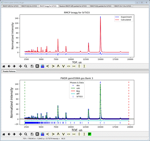
This plot was made by dragging one plot tab to the bottom of the screen to create the second frame.

However if you look at the S(Q) and G(R) plots

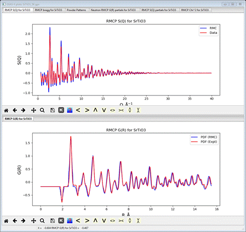
There are clearly two problems. Both plots have an increasing mismatch for higher R and Q; one is the reverse of the other. Secondly, there is a scaling issue especially evident in the S(Q) plot where the data is less than the RMC calculated result. Both of these issues arise from faults in the data processing. The scaling can be corrected in RMCProfile but the peak offset must be fixed first.

Step 8. Fixing peak offset and allow scaling

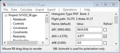
The peak offset in this case arises from different diffractometer constants (especially difC) used for the Rietveld refinement and the processing for F(Q) and G(R). To fix this, one must adjust difC and repeat the Rietveld refinement. This shifts the lattice parameters and ultimately the size of the big box model. To begin select Instrument Parameters under the PWDR entry in the GSAS-II data tree (the plot will change to give resolution curves)

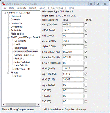
Select the RMCP G(R) for SrTiO3 plot and zoom to the highest R end of the plot (I’ve turned on the plot grid – press ‘g’).

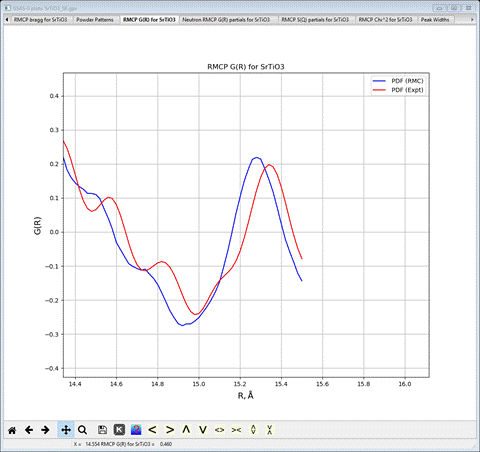
You want to shift the difC value by the ratio of the RMC/Expt (blue curve/red curve) peak positions. You can read these from the plot status bar as you position the cursor on the plot. Enter 6663.06*15.281/15.346 in the difC data field, GSAS-II will do the math and show the result

Next turn off all refinement flags in Instrument Parameters, SrTiO3/Atoms and SrTiO3/Data; then do Calculate/Refine (twice) from the main menu. The residual will be very poor to begin, but will fall to ~7.19% after the second set of refinement cycles.

Now you have to repeat the RMCProfile run starting from a fresh set of lattice parameters and atom positions. This requires a new SrTiO3.rmc6f file. Select the SrTiO3/RMC tab

Pick one of X-axis, Y-axis or Z-axis; change the value to something else and then back so they are 6, 6, and 4 when done. This forces a reset of atom positions and box dimensions. Also select the Fit scale factors option; this is at the beginning of the data processing section. Then do Operations/Setup RMC; the console should show that a new SrTiO3.rmc6f file was written.

Then do Operations/Execute (say Ok to the nag note) to run RMCProfile. As it runs it will report on its console the scale factors for each Expt data set: ~1.14 for G(R) “Expt 1” and ~1.21 for F(Q) “Expt 2”. When completed, the chi^2 values for G(R) (0.6513 vs 2.980) and F(Q) (0.1258 vs 1.899) are much improved while the Bragg fit is essentially unchanged (0.9684 vs 1.003). To see the result do Operations/View; the peaks in the RMCP G(R) for SrTiO3 plot now line up and the scaling issue appears to be resolved although there is an offset between the RMC and Expt curves at low R.

Finally, one can modify the weights to achieve better balance between the three data sets. In the RMC data window change the G(R) weight to 0.02 and the F(Q) one to 0.01; do Operations/Setup RMC to update the RMCProfile files and then do Operations/Execute again for another 10min. My result gave Bragg chi^2 = 0.9619, G(R) chi^2 =1.769 and F(Q) chi^2 = 2.613 which are better balanced.

Step 8. View the big box structural model for SrTiO₃

Next, we can view the resulting big box structure. Do Import/Phase/from RMCProfile .rmc6f file; a FileDialog box with one entry will show the required file, SrTiO3.rmc6f. You will first see a Is this the file you want popup window; select Yes. Next will be an Edit phase name popup. The proposed name is the same as the existing one; GSAS-II will rename this one by adding ‘_1’ to the end. 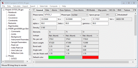Next will be a popup for Add histograms; respond Cancel because you don’t want this phase to be in any subsequent Rietveld refinement. Looking at the General tab for this phase we see it is 6x,6x,4x in all three axes relative to the original and has no symmetry (space group P 1).

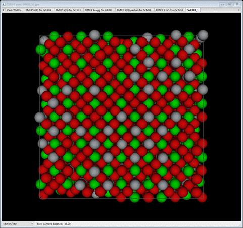
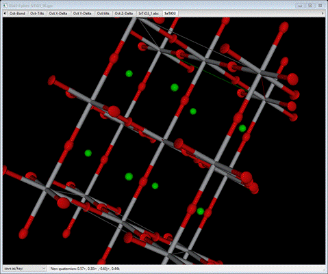
Select the Draw Atoms tab for this phase; a van der Waals ball model will be drawn; scroll out (mouse wheel) to see it more clearly. You should see something like

NB: this import facility can be used to load any rmc6f file, e.g. from a RMCProfile run done outside of GSAS-II; all the plotting and tools in this and the following steps are available for these big box models.

Step 10. Polyhedral comparison for the big box model

In this step we will examine how the suite of TiO₆ octahedra deviate from an ideal octahedron. This analysis is currently restricted to structures with P1 space group symmetry; this is what we have from Step 9 above. Select Phases/SrTiO3_1 from the data tree; the General tab will appear.

What we want is at the bottom of this panel; scroll down to the bottom

At the very bottom is the control for polyhedral comparison. All that is needed is to select the central atom (“origin atom type”) and the polyhedral vertices (“target atom type”). Select Ti for the former and O for the latter. Then do Compute/Compare from the menu; a popup for setting Distance Angle Controls will appear

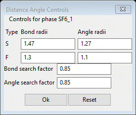
In some cases the bond search factor may need to be adjusted to get the right number of vertices for the polyhedral; in this case 0.85 is too large; change it to 0.79 (NB: in this use the angle ranges are ignored). Press OK; a progress bar will show the atoms being processed. The console will show some atoms being skipped because the number of vertices wasn’t either 4 (tetrahedron) or 6 (octahedron). In this case it takes a while; be patient. The progress bar will show how it is doing; it shows for all atoms and will quickly finish after ~1150 atoms (the end of the Ti atoms). The General tab reappears already scrolled to the bottom

A new button (Show Plots?) has appeared after the atom selections; press it. A number of new entries will appear on the plot window; we will discuss each in turn. Select the Oct-Bond tab

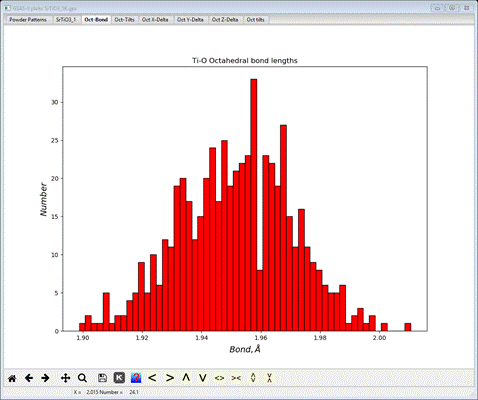
This gives the distribution of Ti-O bond lengths for all the octahedra found across the big box model. It is rough because of the small size of the model (the hole at 1.96 is just a statistical accident). The console will have listed the average value with the standard uncertainty in parentheses.

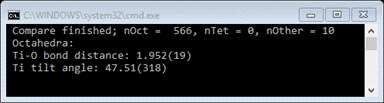
Next select the Oct-Tilts tab

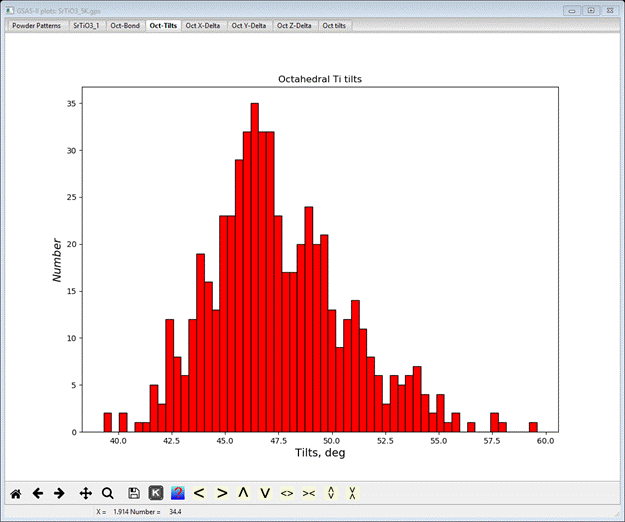
This gives the distribution of axial tilts of the TiO₆ octahedra from the reference octahedron (aligned along the Cartesian axes). There is a wide distribution with a roughly average tilt >45 deg (the average tilt is also shown on the console); in the average perovskite structure this tilt is exactly 45 deg so there is a subtle twist of the octahedra of ~2.5 deg from the average. Next select Oct X-Delta, Oct Y-Delta and Oct Z-Delta tabs in turn.

I have made this plot by dragging the respective plot tabs to one of the right (or left) edges to create a 3 pane plot. These show the displacement of the O atoms from the ideal octahedral vertices along each Cartesian axis. Here they are arranged about the zeros fairly tightly. If there were structural distortions to the octahedra (e.g. Jahn-Teller distortions) these could show in these plots. Finally select the Oct tilts tab; a 3D plot will be shown

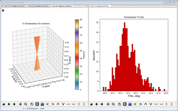
What we see here is a fan of unit vectors along the z-axis all with about the same color consistent with the tilt angles shown in the right hand panel. About half are along +Z and the other half along –Z and tipped slightly about the Y-axis.

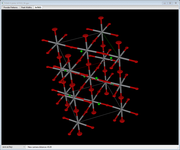
Step 10. View the disordered average structure

We can compress the big box result back into the original average crystal structure to see how the disordered sites compare with the average ones. Select the General tab for the big box phase (SrTiO3_1) and then do Compute/Transform. A popup dialog will appear

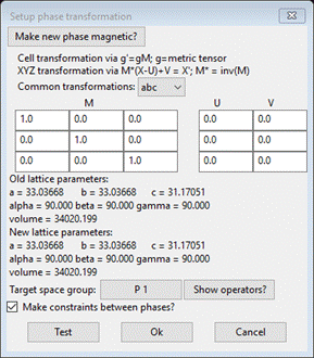
This is the general tool inside GSAS-II for all sorts of structure transformations. Here we will use it to push all the big box atoms back into the average structure unit cell. Recalling that the big box model is 6x6x4 the original unit cell, we simply want to reverse the process. Enter 1/6, 1/6, 1/4 into the diagonal elements of the M matrix. The GUI will convert them to the decimal equivalent (0.1666… and 0.25). The target space group should be P 1. Press the Test button; you should see

Press Ok to do the transformation. A new phase, “SF6_1 abc” will be formed as triclinic with cell axes that match the original tetragonal ones. Select Draw Atoms; a van der Waals model will appear.

Select the Draw Options tab and reduce the van der Waals scale to about 0.05.

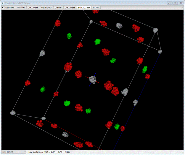
This compares pretty well with the original structure with the ellipsoids drawn at 99% probability.

Although it doesn’t quite capture the pancake appearance of some of the O-atom thermal motion.

Final note

The problem with the value of the difC diffractometer constant means that there is an unknown small bias in the scale of G(R) and thus all interatomic distances. This is only resolved by careful calibration of the diffractometer via known standards using the profile functions known to both RMCProfile and GSAS-II and the universal use of those parameters for all data reduction steps for both the powder pattern and the F(Q) and G(R) data sets.