This tutorial has three sections:
The first section duplicates the refinement in the GSAS-II CW Combined Refinement tutorial as a multi-step process. The second section repeats the previous refinement, but demonstrates how a complex process can be entered into a single Python dict and the refinement executed with a single function call. The third section shows how a pattern simulation, rather than refinement can be executed from a script.
The exercise can be performed by placing all of the Python commands
into a script,
but a more pedagogical approach will be to enter the
commands into a Python interpreter. Use of IPython or Jupyter to run
Python will make this a more pleasant experience.
A. Create a Multi-step Script
Note that the script in this section is supplied for
download here, but some editing will be needed to match where files
are found on your computer.
The first step in writing any Python module is to load the modules that will be needed. Here we will need the os and sys modules from the Python standard library and the GSASIIscriptable from the GSAS-II code. The location where the GSAS-II source code is installed must usually be hard-coded into the script as is done in the example below. Note that a common location for this will be os.path.expanduser("~/g2conda/GSASII/") or '/Users/toby/software/GSASII', etc. Thus the script will begin with something like this: If a ImportError: No module named GSASIIscriptable error occurs, then the wrong directory location has been supplied for the GSAS-II files.
To simplify this example, we will define the location where files will be written as workdir (this directory must exist, but it may be empty) and the location where the input files for this exercise ("PBSO4.XRA", "INST_XRY.PRM", "PBSO4.CWN", "inst_d1a.prm" and "PbSO4-Wyckoff.cif") will be found as datadir. (As discussed previously, these files can be downloaded from here. )We also define here a short function to display the weighted profile R factor for every histogram in a project, HistStats. This will be discussed later.
The first step in creating a GSASIIscriptable script to to create or access a GSAS-II project, which is done with a call to GSASIIscriptable.G2Project(). This can be done in one of two ways: a call with G2sc.G2Project(newgpx=file) creates a new (empty) project, while a call with G2sc.G2Project(gpxfile=file) opens and reads an existing project (.gpx) file. Both return a G2Project wrapper object that is used to access a number of methods and variables. Note that GSASIIscriptable.G2Project() can read .gpx files written by both previous GSASIIscriptable.G2Project() runs or the GSAS-II GUI.In this example, we create a new project by using the newgpx=file argument with this code:
Note that the file will not actually be created until an operation that saves the project is called.
To add two powder diffraction datasets (histograms) and a phase to the project using this code: We use the project.add_powder_histogram() method in the GSASIIscriptable class to read in the powder data. The two arguments to .add_powder_histogram() are the powder dataset and the instrument parameter file. Note that these files are both "GSAS powder data" files and the importer for this format (and many others) allows files with arbitrary extensions to be read. All importers that allow for extensions .XRA and .CWN will be used to attempt to read the file, producing a number of warning messages. To specify that only the GSAS powder data importer be used, include a third argument, fmthint="GSAS powder" or something similar (fmthint="GSAS" is also fine, but will cause both the "GSAS powder data" and the "GSAS-II .gpx" importer to be considered.)
- Note that project.add_powder_histogram() returns a powder histogram objects, which here are saved for later reference. It is also possible to obtain these using gpx.histograms(), which returns a list of defined histograms.
Then we add a phase to the project using project.add_phase(). This specifies a CIF containing the structural information, a name for the phase and specifies that the two histograms are "added" (linked) to the phase. The fmthint="CIF" parameter can also optionally be specified to limit the importers that will be tried.
- Note that project.add_phase() returns a phase object
- Also, the previously saved histogram objects are used in the project.add_phase() call. Note that it is also possible to reference the two histgrams by their numbers in the project (here histograms=[0,1]) or by the histogram names (here
histograms=['PWDR PBSO4.XRA Bank 1', 'PWDR PBSO4.CWN Bank 1']). These three ways to use the histograms parameter produce the same result.
While this is not noted in the original tutorial, this exercise will not complete properly if more variables are added to the refinement without converging the refinement (or at least coming close to convergence) at each refinement step. This is best accomplished by increasing the number of least-squares cycles. No supplied method (at present) allows this parameter to be set straightforwardly, but this code will do this:To find this parameter in the GSAS-II data structure, I followed these steps: In the GUI, Controls is the tree item corresponding to the section where Least Squares cycles are set. Executing the command gpx.data.keys() shows the names of the entries in the dictionary corresponding to the GSAS-II tree and indeed one entry is 'Controls'. Command gpx.data['Controls'].keys() shows that all values are located in an entry labeled 'data' and gpx.data['Controls']['data'].keys() shows the entries in this section. Examination of gpx.data['Controls']['data']['max cyc'] shows the value 3, which is default number of cycles. Thus, the number of cycles is changed with the Python command above.
In Step 4 of the original tutorial, the refinement is performed with the variables that are on by default. These variables are the two histogram scale factors and three background parameters for each histogram (8 in total). With GSASIIscriptable, the background refinement flags are not turned on by default, so a dictionary must be created to set these histogram variables. This code:Function HistStats() works by using gpx.histograms() to iterate over all histograms in the project, setting hist to each histogram object. Class member hist.name provides the histogram name and method hist.get_wR() looks up the profile R-factor and prints them. The function also writes the final refinement results into the current project file. The output from this will be:
- defines a dictionary (refdict0) that will be used to set the number of background coefficients (not really needed, since the default is 3) and sets the background refinement flag "on".
- The project is saved under a new name, so that we can later look at the results from each step separately.
- The parameters in refdict0 are set using project.do_refinements() for both histograms in the project and the a refinement is run.
- The weighted profile R-factor values for all histograms in the project are printed using the previously defined HistStats() function.
Note that the Rwp values agree with what is expected from the original tutorial.Hessian Levenburg-Marquardt SVD refinement on 8 variables: initial chi^2 9.6912e+06 Cycle: 0, Time: 1.88s, Chi**2: 6.7609e+05, Lambda: 0.001, Delta: 0.93 initial chi^2 6.7609e+05 Cycle: 1, Time: 1.84s, Chi**2: 6.7602e+05, Lambda: 0.001, Delta: 0.000104 converged Found 0 SVD zeros Read from file: /Users/toby/software/G2/Tutorials/PythonScript/step4.bak0.gpx Save to file : /Users/toby/software/G2/Tutorials/PythonScript/step4.gpx GPX file save successful Refinement results are in file: /Users/toby/software/G2/Tutorials/PythonScript/step4.lst ***** Refinement successful ***** *** profile Rwp, step4.gpx PWDR PBSO4.XRA Bank 1: 40.88 PWDR PBSO4.CWN Bank 1: 18.65Note: that there are several equivalent ways to set the histogram parameters using G2PwdrData.set_refinements(), G2Project.set_refinement() or my_project.do_refinements(), as described here. Thus, the gpx.do_refinements([refdict0]) statement above could be replaced with:
orgpx.set_refinement({"Background": { "no. coeffs": 3, "refine": True }}) gpx.do_refinements([{}])for hist in gpx.histograms(): hist.set_refinements({"Background": { "no. coeffs": 3, "refine": True }}) gpx.do_refinements([{}])
In Step 5 of the original tutorial, the refinement is performed again, but the unit cell is refined in the phase. In this case the gpx.set_refinement(refdict1) statement can be replaced with:Note that it is also possible to combine the refinement in the current and previous section usingphase0.set_refinements({"Cell": True})but then the results are not saved in separate project files and it is not possible to see the Rwp values after each refinement.gpx.do_refinements([refdict0,refdict1])
In Step 6 of the original tutorial, the refinement is performed again after adding Histogram/Phase (HAP) parameters so that the lattice constants for the first histogram (only) can vary. This is done with this code: Here we cannot use gpx.do_refinements([refdict2]) with refdict2 defined as above because that would turn on refinement of the Hstrain terms for all histograms and all phases. There are several ways to restrict the parameter changes to specified histogram(s) and phase(s). One is to call a method in the phase object(s) directly, such as replacing the gpx.set_refinement(...) statement with this:It is also possible to add "histograms" and/or "phases" values into the refdict2 dict, as will be described below.phase0.set_HAP_refinements({"HStrain": True},histograms=[hist1])
The next step in the original tutorial is to treat sample broadening by turning on refinement of the "Mustrain" (microstrain) and "Size" (Scherrer broadening) terms using an isotropic (single-term) model. As described in the documentation for Histogram/Phase parameters, type must always be specfied even as in this case where it is not being changed from the existing default. Again, since these parameters are being set only for one histogram, either phase0.set_HAP_refinements() or gpx.set_refinement() must be called or to use gpx.do_refinements([refdict3]) the "histograms" element must be included inside refdict3.
The step 8 in the original tutorial is to treat sample displacement for each histogram/phase. These parameters are different because of the differing diffractometer geometries. We also add refinement of sample parameters using phase0.set_refinements() to set the "X" (coordinate) and "U" (displacement) refinement flags for all atoms. This is done with this code: Note that the original tutorial calls for the diffractometer radius to be changed to the correct value so that the displacement value is in the correct units. This parameter cannot be set from any GSASIIscriptable routines, but following a similar process, as before, the location for this setting can be located in the histogram's 'Sample Parameters' section (as hist2.data['Sample Parameters']['Gonio. radius']). Also note that the settings provided in the phase0.set_refinements() and statements gpx.do_refinements() could have been combined into this single statement:gpx.do_refinements({"set":{"Atoms":{"all":"XU"}})
The final step in the original tutorial is to trim the range of data used in the refinement to exclude data where no reflections occur and where the peaks are cut off at high angle. Also, additional parameters are refined here because the supplied instrumental profile parameters are not very accurate descriptions for the datasets that are used here. It is not possible to refine the Lorentzian x-ray instrumental broadening terms, since this broadening is treated as sample broadening. The Lorentzian neutron broadening is negligible. Note that the final gpx.do_refinements() statement can be replaced with calls to histX.set_refinements() or gpx.set_refinement(), such ashist1.set_refinements({'Instrument Parameters': ['U', 'V', 'W']}) hist2.set_refinements({'Instrument Parameters': ['U', 'V', 'W']}) gpx.do_refinements([{}])
As is noted in the GSASIIscriptable module documentation, the project.do_refinements() method can be used to perform multiple refinement steps. Note that this version of the exercise can be downloaded here. To duplicate the above steps into a single call, a more complex set of dicts must be created, as shown below: Note that above the "call" and "callargs" dict entries are defined to run HistStats and "output" is used to designate the .gpx file that will be needed. When parameters should be changed in specific histograms, the entries "histograms":[hist1] and "histograms":[hist2] are used (equivalent would be "histograms":[0] and "histograms":[1]). Since there is only one phase present, use of "phase":[0] is superfluous, but in a more complex refinement, this could be needed.A list of dicts is then prepared here:
Steps 4 through 10, above then can be performed with these few commands:
Use of the GSASIIscriptable module makes it very simple to simulate a powder diffraction pattern using GSAS-II. This is demonstrated in this section. Note that the Python commands can be downloaded here.As before, the location of the GSASIIscripts Python module must be defined and the module must be loaded:
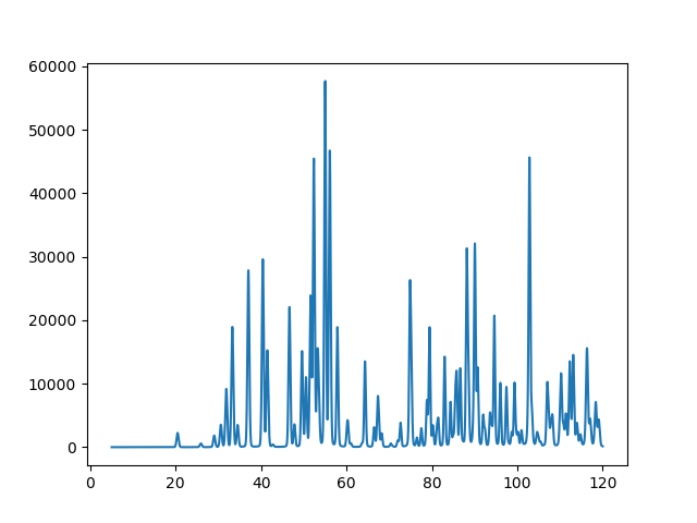
To simplify this example, as before we will define the location where files will be read from and written (as datadir and workdir). Note that files "inst_d1a.prm" and "PbSO4-Wyckoff.cif" from here are needed. We then need to create a project and for this example we choose to define the phase first. (It would work equally well to create the histogram first and then define the phase.) We then add a "dummy" histogram to the project. Note that an instrument parameter file is specified, but not a data file. The range of data to be used and the step size must be specified. The phases parameter is specified as ``gpx.phases()`` which creates a list of all the previously read phases, which in this case is equivalent to ``[phase0]``. Note that the computed pattern cannot be seen above "simulated noise" unless the intensities are large enough. We can change the pattern scale factor using the Scale factor (parameter hist1.data['Sample Parameters']['Scale'][0]), as shown below. Next, to perform the simulation computation, a refinement is needed: However, there is no need to actually optimize any variables, so the number of refinement cycles is set to zero. Refinement is initiated then with proj.do_refinements. To keep the results in a .gpx file, the project is saved.Finally, we want to do something with the results. The histogram could be written to a file with the histogram.Export() command. Note that the first time a refinement computation is done with a dummy histogram the "observed" pattern is set from the calculated intensities. Here an alternate option is used, where the values are retrieved and plotted.
Note that in the above, gpx.histogram(0) is used to show how to reference hist1 when the histogram object is not known. The generated two-theta values and computed intensity values are retrieved and the remaining lines generate a very simple plot which is saved to a file, as shown below.