PDFfit-IV
Introduction
In these
tutorials, we will show how to use GSAS-II in conjunction with PDFfit2
(“PDFfit2 and PDFgui: computer programs for studying
nanostructures in crystals", C.L. Farrow, P.Juhas,
J.W. Liu, D. Bryndin, E.S. Bozin,
J. Bloch, Th. Proffen & S.J.L. Billinge, J. Phys, Condens.
Matter 19, 335219 (2007), Jour. Phys.: Cond. Matter (2007), 19, 335218. doi: https://doi.org/10.1088/0953-8984/19/33/335219) to fit
pair distribution functions (PDF) with a “small box” disordered model. We will
refer to PDFfit2 as “PDFfit” in these tutorials as
well as in the GSAS-II user interface for it.
The
GSAS-II interface to PDFfit is a simplification where
some capabilities of PDFfit are not implemented;
GSAS-II only allows a single phase for PDFfit and the
atom thermal displacement model is strictly isotropic. PDFfit
allows multiple phases and anisotropic thermal motion; we considered these to
be not useful and an unneeded complication, and these are better tackled via
Rietveld refinement with the original diffraction data.
We
have included with the GSAS-II distribution the most recent version of the
PDFfit2 executable and its python interface routines for Windows (those for Mac
OSX and linux will follow in due course). They are in
the diffpy subdirectory of GSAS-II. No
other files are needed. Also, the diffpy/manual subdirectory has the paper referenced above as well as one
that described the original Fortran version of PDFfit.
PDFgui.html describes 3 tutorials, upon
which the GSAS-II ones are based, as given for the PDFgui
software. Alternatively, you can install pdffit2 from Anaconda by executing
conda install -c diffpy diffpy.pdffit2
in a console
window after activating your version of python.
It will be installed in your python as gsas2full/Lib/site-packages/diffpy.
In
this tutorial we will compare analysis for bulk and nanoparticle CdSe using x-ray G(r) patterns taken at 6-ID-D of the
Advanced Photon Source to introduce you to the process of doing PDFfit analysis within GSAS-II for nanoparticles. If you
haven’t done so already, start GSAS-II.
Step 1. Setup
parent CdSe phase
The
blank startup view of GSAS-II begins with this
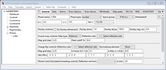
The
structure of CdSe is quite simple; space group P 63mc,
a=4.3Å, c=7.01Å with Cd at 1/3, 2/3, 0 and Se at 1/3, 2/3, 3/8.
To
begin, do Data/Add new
phase
from the main menu. Call the new phase CdSe and then the General tab
will appear
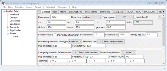
Enter
the space group, P 63 m c (don’t forget the spaces);
the window will repaint. Fill in the a (4.3) and c (7.01) lattice parameters; the window should show
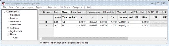
Next,
select the Atoms tab (it will be empty) and
do Edit Atoms/Append atom twice. Change the 1st
atom Type to Cd & the 2nd to Se (each time a periodic table will appear). Then change the
atom positions to 1/3, 2/3, 0 for the Cd and 1/3, 2/3, 3/8 for the Se (fractions are ok
– GSAS-II converts them to double precision floats). When done, the window
should show
Step 2. Setup the
bulk and nano-crystalline forms of CdSe for PDFfit
Because
PDFfit works only on the full unit cell contents, we
need to create new phases of CdSe for the bulk and
nano forms. We will use the Transform tool in GSAS-II to do this. Select the General tab for the CdSe phase and then
do Compute/Transform; a popup dialog will appear
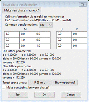
Change
the Target space group to P 1 (press Ok twice to get back to the dialog); then press Ok. The General tab for the new phase “CdSe
abc” will be shown
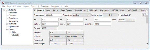
Change
the Phase name to CdSe-bulk; the entry in the tree will change. This will be the phase
to be used for PDFfit on the data from a bulk sample
of CdSe.
Next,
select the original CdSe phase and repeat the Compute/Transform; again, change the Target
space group to P 1 and press Ok (3 times). The new phase will be displayed; change its name
to CdSe-nano. When done you should see
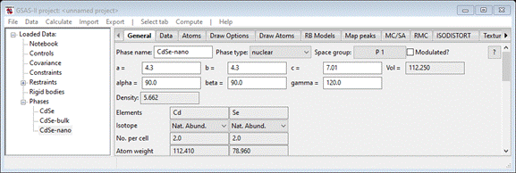
and
we are ready to do PDFfits to the respective bulk and
nano CdSe data. This is a good time to save your
project (I called it simply CdSe)
Step 3. PDFfit of bulk CdSe
We
begin with the bulk CdSe first as that will give us
some baseline parameters to compare the nano CdSe
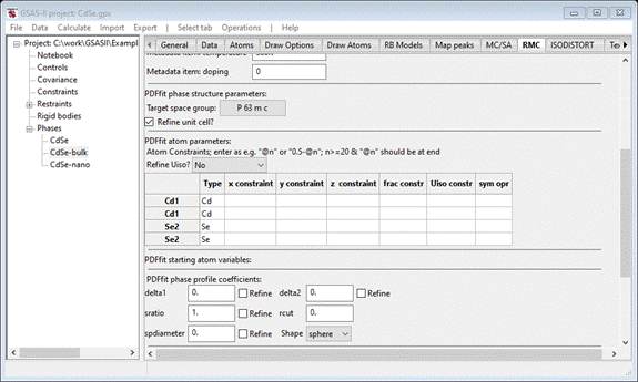
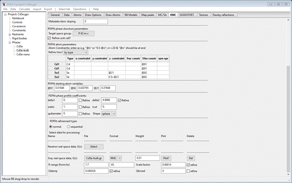
with. Select the CdSe-bulk phase and pick the RMC tab. Then select the PDFfit radio button. The window
will refresh to show the PDFfit setup
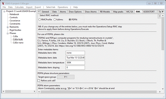
Change
the Target space group to P 63 m c; this will determine the
symmetry restrictions on the unit cell. Check the Refine unit cell box. The middle of the
window will show the atoms filled in
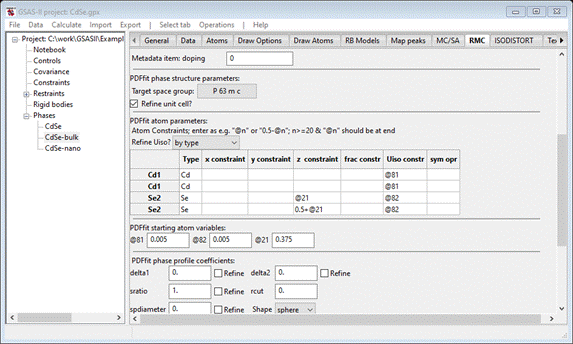
For
Refine Uiso select by type; the window will repaint showing @81 and @82 as Uiso constraints for the Cd and Se atoms, respectively.
Enter @21 in the 1st Se2 z
constraint; the window will repaint. Then enter 0.5+@21 for the 2nd Se2 z
constraint. Finally enter 0.375 in the @21 PDFfit starting atom variables box. When done the window
should look like
Next
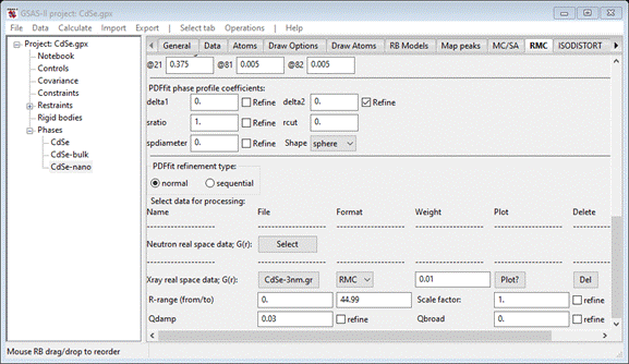
check the delta2 Refine box. Then press the X-ray
real space data; G(r) Select button; a file dialog box
will appear. Navigate to PDFfit-IV/data and select CdSe-bulk.gr; the window will repaint to
show
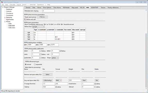
Change
R-range “from” to 1.7 and check the refine boxes for Scale factor and Qdamp.
This completes the setup for the PDFfit on bulk CdSe.
To
run PDFfit, you first must prepare its input files;
do Operations/Setup RMC. A few lines will appear on
the console. Then do Operations/Execute; a popup will appear as a
reminder to cite PDFfit2. Press OK; new console window will
appear showing the output from PDFfit. At the end it
will show the residual (Rw = 0.18) along with a list
of the final results; press any key. The console will vanish,
and a small popup will appear
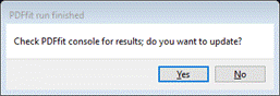
Since
the result was ok, press Yes; the window will be updated
with the new values. If you repeat the two steps (Operations/Setup RMC and Operations/Execute) PDFfit
will be rerun with new parameters; there will be a slight improvement in the
fit (Rw = 17%) and the window will show
The
value of Qdamp (0.049326) is considered to be
characteristic of the instrument used to collect the original diffraction data
used to produce this pdf; we will use it as a fixed value in the analysis of
nano-CdSe described in the next step below.
If
you next do Operations/Plot, the resulting fit to the
data will be shown
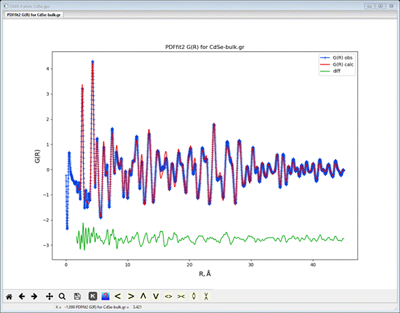
Not
a bad fit. You should save your project before proceeding to the next step.
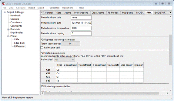
Step 4. PDFfit of nano CdSe
In
this step we will repeat the sequence of operations we used for bulk CdSe except we will explore using PDFfit
to determine the nanoparticle diameter. To begin, select the CdSe-nano phase and its RMC tab; it may display the PDFfit page, if not select the correct radio button. It
will show
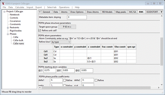
As
before, change the space group to P 63 m c, check the Refine unit cell box and enter @21 for the 1st Se2 z constraint and 0.5+@21 for the 2nd one.
Also select Refine Uiso by type. Enter 0.375 for the @21 variable. This
should give
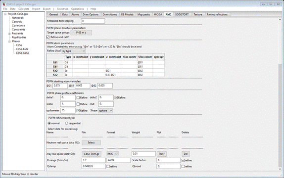
Next
check the delta2 Refine box. Then press Select for X-ray real space data. Navigate to PDFfit-IV/data and select CdSe-3nm.gr; the window will repaint
Change
R-range (from) to 1.7 and check the refine for Scale factor but not Qdamp;
set Qdamp to 0.049326 the value obtained from the
analysis of bulk CdSe. The key parameter for
nanoparticles is their diameter; this is the parameter “spdiameter”.
Set it to 25 and check its Refine box. The window should look like
Now
we are ready to try to fit it. Do Operations/Setup
RMC and
then Operations/Execute; after responding to the
“nag” note a new console will appear. The refinement converges poorly (Rw=56%), but let’s accept it anyway. Then do Operations/Setup RMC and Operations/Execute again. This time the
refinement improved to Rw=30%. Accept it and then do Operations/Plot to see the fit
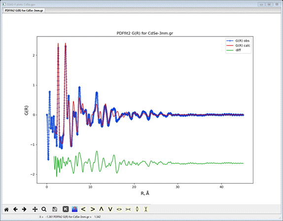
The
calculated pdf fits the first two peaks (closest Cd-Se and Cd-Cd, Se-Se
distances) quite well but poorly for larger distances; our simple model is
insufficient but notice how the pattern fades out at ~30Å compared to that for
bulk CdSe. The refined value for spdiameter
is 27.3Å consistent with our expectations. This concludes this PDFfit tutorial; you can save the project if you wish. A
perhaps useful paper on this material can be found at http://link.aps.org/doi/10.1103/PhysRevB.76.115413
(you’ll probably need access via your library to see it).