PDFfit-III

Exercise files are found here

Introduction

In these tutorials, we show how to use GSAS-II in conjunction with PDFfit2 (“PDFfit2 and PDFgui: computer programs for studying nanostructures in crystals", C.L. Farrow, P.Juhas, J.W. Liu, D. Bryndin, E.S. Bozin, J. Bloch, Th. Proffen & S.J.L. Billinge, J. Phys, Condens. Matter 19, 335219 (2007), Jour. Phys.: Cond. Matter (2007), 19, 335218. doi: https://doi.org/10.1088/0953-8984/19/33/335219) to fit pair distribution functions (PDF) with a “small box” disordered model. We will refer to PDFfit2 as “PDFfit” in these tutorials as well as in the GSAS-II user interface for it.

The GSAS-II interface to PDFfit is a simplification where some capabilities of PDFfit are not implemented; GSAS-II only allows a single phase for PDFfit and the atom thermal displacement model is strictly isotropic. PDFfit allows multiple phases and anisotropic thermal motion; we considered these to be not useful and an unneeded complication, and these are perhaps better tackled via Rietveld refinement with the original diffraction data.

We have included with the GSAS-II distribution the most recent version of the PDFfit2 executable and its python interface routines for Windows (those for Mac OSX and linux will follow in due course). They are in the diffpy subdirectory of GSAS-II. No other files are needed. Also, the diffpy/manual subdirectory has the paper referenced above as well as one that described the original Fortran version of PDFfit. PDFgui.html describes 3 tutorials, upon which the GSAS-II ones are based, as given for the PDFgui software. Alternatively, you can install pdffit2 from Anaconda by executing

conda install -c diffpy diffpy.pdffit2

in a console window after activating your version of python. It will be installed in your python as gsas2full/Lib/site-packages/diffpy.

In this tutorial we will continue the analysis LaMnO₃ using variable temperature neutron G(r) patterns to introduce you to the process of doing sequential PDFfit analysis of mode distortions within GSAS-II. At the end you will be able to step through the sequence and see how the structure responds to temperature change from 300K to 980K. If you haven’t done so already, start GSAS-II.

If you have already done the PDFfit-II tutorial and have retained the result from ISODISTORT (LaMnO3-Pbnm_child.cif), you can skip Steps 1 & 2 and go directly to Step 3, because these duplicate your operations in that tutorial to yield this cif file.

Step 1. Setup LaMnO₃ Pbnm phase

The blank startup view of GSAS-II begins with this

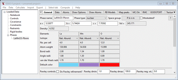
First, we need a description of the expected LaMnO₃ structure (probably generated from a powder or single crystal structure determination); this is in the data package for this tutorial. Do Import/Phase/from CIF file. A file dialog box will appear. Navigate to PDFFIT-III/data and select LaMnO3 Pbnm.cif. Respond Yes to the file check box and accept the phase name as given. The General tab will appear

If desired, you can examine the 4 atom positions and make a drawing by following the operations as outlined in the previous tutorial.

Step 2. ISODISTORT analysis of LaMnO₃

If you access the ISODISTORT web site directly via https://iso.byu.edu/iso/isodistort.php, it will take you through a sequence of web pages with many possible alternatives to choose from, but it always begins with an undistorted high symmetry parent structure. We have reduced all this to a single preselected step that compares a given structure (e.g. this LaMnO₃ Pbnm phase) and compares it to the undistorted parent phase and determines the possible distortion modes and their magnitudes (ISODISTORT Method 4). 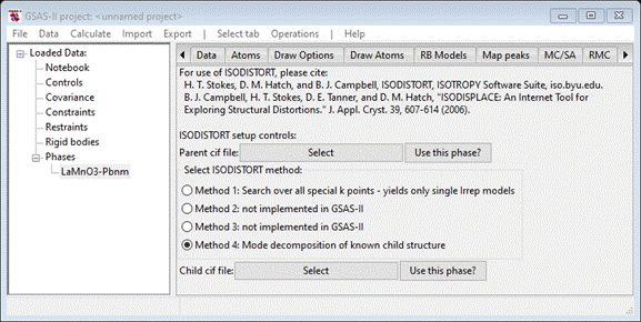This operation results in a cif file containing all the information required by GSAS-II to construct a mode refinement model. To begin select the ISODISTORT tab for the LaMnO₃-Pbnm phase; you should see

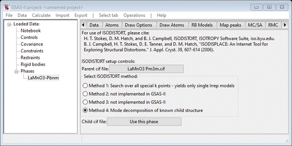
Press the “Parent cif file” Select button; a file selection dialog will appear. Navigate to PDFFIT-III/data and select LaMnO3 Pm3m.cif. The window will repaint to show the choice (note that this does not import this phase into GSAS-II). Since we have already imported the Pbnm phase of LaMnO₃ and are working out of its ISODISTORT tab, we can use it for the “Child cif file”. Press Use this phase? The window will repaint giving the two choices.

We are now all set to run ISODISTORT; you must be connected to the internet for this to work as we are remotely accessing the https://iso.byu.edu/iso/isodistort.php web page and all that follows (about four more pages). Do Operations/Run ISODISTORT; the console will show a series of messages as GSAS-II accesses various web pages at the ISODISTORT site. It will successfully finish with a popup message

Press OK; the console will display a final message

indicating that a new cif file (LaMnO3-Pbnm_child.cif) has been created. This contains all the constraint information needed to construct them in GSAS-II.

Step 3. Import and examination of ISODISTORT result

If you still have LaMnO3-Pbnm_child.cif from the PDFfit-II tutorial, you can start here. Do Import/Phase/from cif file; a file dialog box will appear. There will be (at least) 2 files. One is the one created for input to ISODISTORT (ISOin.cif) and the other is the result from ISODISTORT, LaMnO3-Pbnm_child.cif. Select it; respond Yes to the popup file check and leave the phase name as it is. The console will display several messages as GSAS-II interprets the content of the cif file and develops the appropriate constraints to make the distortion modes as GSAS-II variables. These are then displayed in the ISODISTORT tab

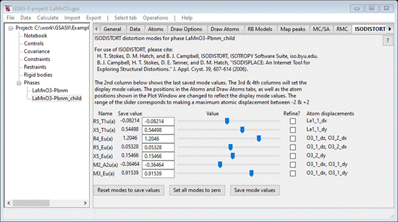
Shown are the 7 displacement modes (NB: the same number as the number of independent atom coordinates in this Pbnm perovskite), their values in Angstroms and at the end the atom coordinates involved in each one. If you began with the LaMnO3-Pbnm_child.cif file from PDFfit-II tutorial skipping Steps 1 & 2, there will only be one phase in the project.

To see how the various modes change the structure, you must draw it first; this will be useful to have when you examine the structure to see how it changes with temperature. (Trying the sliders now will give you an error message). Select the Draw Atoms tab

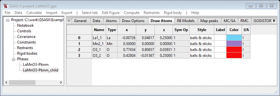
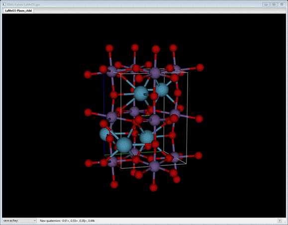
Select all atoms, do Edit Figure/Fill unit cell. Then left double click Type and select Mn; then do Edit Figure/Fill CN-sphere. You should see (after a bit of rotation)

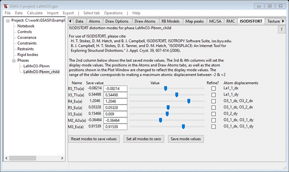
Now select the ISODISTORT tab. You can now shift the sliders to see what each mode does to the structure. When done, press the Reset modes to save values to recover the original structure. The tab should look like

This would be a good time to save the project (do File/Save project); use a name that is different from the one used in the PDFfit-II tutorial (I used LaMnO3 seq.gpx).

Step 4. Setup for PDFfit

We now need to convert this phase (LaMnO3-Pbnm_child) into one that is setup for PDFfit. This process creates a new phase with the constraints transformed into PDFfit constraints. From the ISODISTORT tab, Do Operations/Make PDFfit phase; the window repaints with the ISODISTORT tab still selected

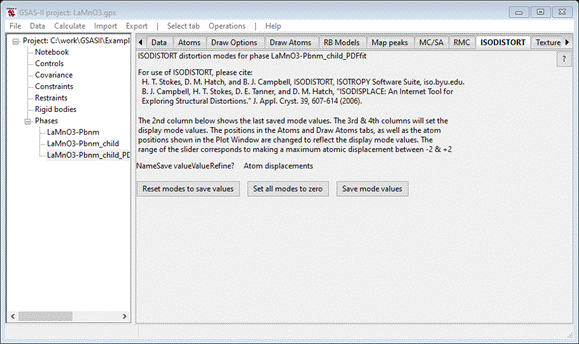
This is now the third phase (LaMnO3-Pbnm_child_PDFfit); the mode information has been transferred. Select the RMC tab and choose the PDFfit radio button; the window now displays the full suite of atom PDFfit position constraints as developed from the ISODISTORT displacement modes.

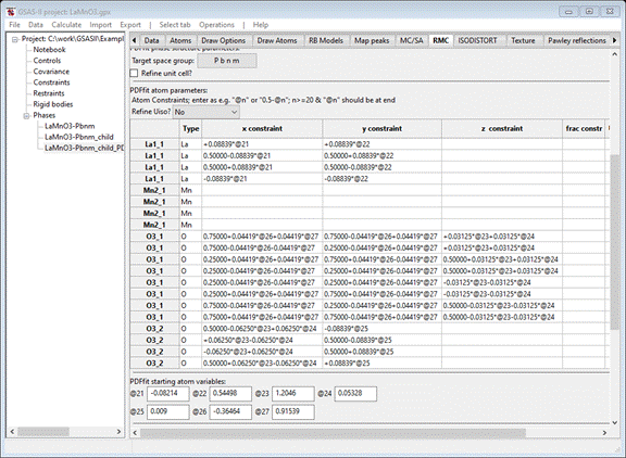
The atom variables (“@21”, etc.) correspond directly with the ISODISTORT distortion modes shown for the LaMnO3-Pbnm_child phase; their values are shown as well. The correct target space group is given (P b n m); you should check the Refine unit cell? box. You should also choose a Uiso refinement model. I selected Refine Uiso ? by parent name, that gives 4 additional parameters (“@81” – “@84”) with starting values (Uiso=0.005) as listed. As with the two earlier tutorials, change “delta2” to 1.0 and check its Refine box. When done the RMC tab should look like

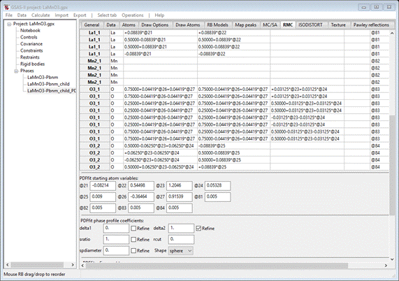
Because the only phase needed for the rest of this tutorial you can delete the others; do Data/Delete phase entries from the main menu. A popup will appear

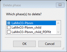
Select the 1^st two items & press OK. The window will be repainted showing only one phase in the data tree

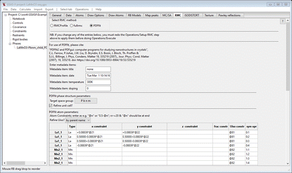
Save the project. (I had used LaMnO3 seq.gpx)

Step 5. Reading sequential PDF data for LaMnO₃ into GSAS-II and sequential PDFfit setup

The sequential PDFfit operation requires that the G(r) data be given as a suite of “PDF” entries in the GSAS-II tree. Do Import/PDF G(R) Data/from r(A) step G(r) data file; a file selection dialog will appear. Navigate to PDFfit-III/data and select all 11 gr files; the window should show all 11 entered in the tree. (Notice that I have deleted the other two phases).

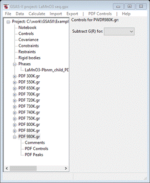
The plot may show G(r) for the last one read.

Now select the LaMnO3-Pbnm_child_PDFfit phase; it should show the RMC tab with PDFfit selected. The bottom of this window should show

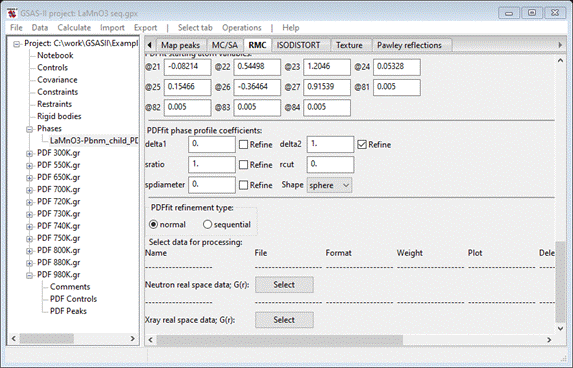
Select sequential for the PDFfit refinement type; the window will be redrawn. The bottom now shows

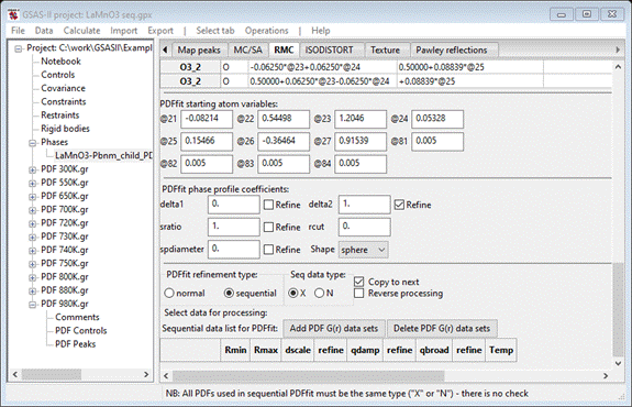
Change Seq data type to ‘N’ and then press the Add PDF G(r) data sets button; a popup dialog will appear

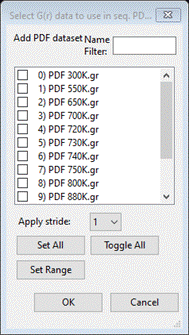
Press Set All and OK; the window will be redrawn showing a table of the data sets at the bottom

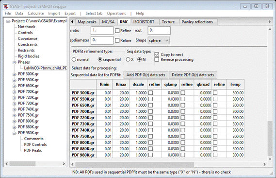
Unfortunately, the data sets did not (apart from the file name) contain a temperature record. You’ll have to enter them by hand. Notice the fine stepping in temperature around 700-750K; this was to track some special structural change in this material. We will be keen to see what comes out of the mode displacements.

We need to set Rmin to 2.0; double click on the Rmin column heading. A small popup will appear; set the value to 2.0 & press OK. The window will be redrawn. Now do the same with the refine column headings for dscale and qdamp selecting Y – vary all in each case. The window is refreshed each time (you’ll have to scroll back down to the bottom each time). When done, this part of the window should look like

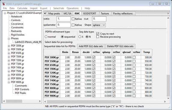
Note the Copy to next box is checked; this facilitates the initial sequential refinement. This finishes the initial setup for a sequential fit using PDFfit. You should save the project.

Step 6. Sequential distortion mode PDFfit for LaMnO3 with temperature

To begin, we must setup the for the sequential PDFfit run. Do Operations/Setup RMC; a short message will appear on the console indicating that Sequential_PDFfit.py written; this is the python script that will drive PDFfit.

Next, do Operations/Execute; a popup will appear reminding you to properly cite your use of PDFfit (don’t forget to cite GSAS-II as well). Press OK. A sequence of consoles will appear, one for each execution of PDFfit. A progress bar will show

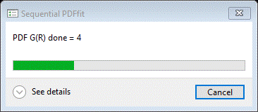
Most steps will be quick (a few seem to require more cycles to converge), but all will show Rw ~ 10%. When finished, the progress bar will vanish, and the sequential result is shown

Step 7. Examination of sequential PDFfit result

There are many ways to examine a sequential result in GSAS-II. Simplest is to select a column heading; the plot will show the parameter as a function of run number (I picked 11-a – the unit cell axis a).

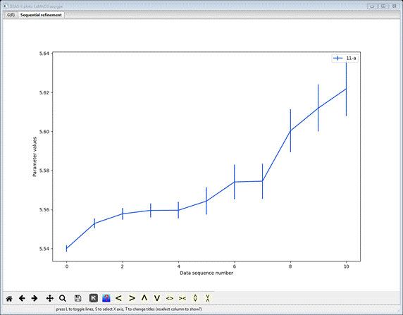
The vertical bars represent the standard uncertainties for each a-axis determination by the sequential PDFfit. Select the plot window and press the ‘s’ key; a small popup window will appear

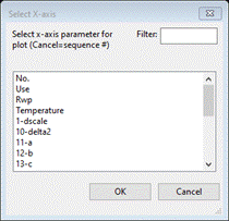
Select Temperature and press OK; the plot will be redrawn with sample temperature as the x-axis

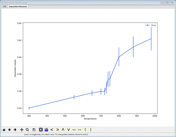
This is considerably more informative. Something interesting seems to be happening at ~750K. Now select all the mode distortion parameters – pick 21-R5_T1u(a) and then hold the Ctrl key down while you pick the rest (to 27-M3_Eu(a)); the plot will show

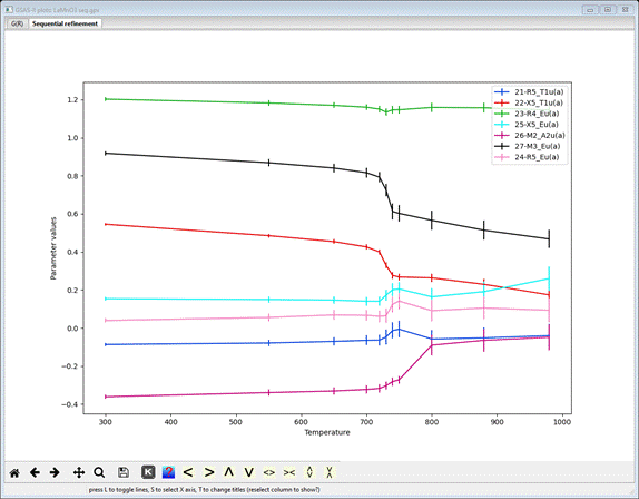
Clearly the anomaly on the a-axis lattice parameter is coincident with distinct transitions in most of the mode distortions. The other thing to note is the trend toward zero for all but the R4_Eu(a) (green curve) mode; it remains essentially constant over the entire temperature range. The convergence of some of the modes prestages the orthorhombic to rhombohedral phase transition at ~1000K for which there are fewer possible distortion modes.

To see the effect of these modes on the structure, GSAS-II allows one to step through the sequence while viewing the crystal structure. Select the Draw Atoms tab for this phase. Then fill it out using the Fill unit cell and Fill CN-sphere commands. The initial view may be

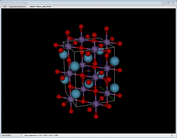
which is the undistorted parent LaMnO₃ cubic perovskite transformed to the orthorhombic Pbnm lattice. Now press the +/= key; the drawing will change to show the effect of the distortion modes at 550K (see message at bottom of plot)

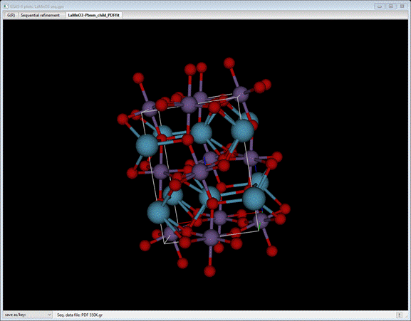
Continue to press the +/= key (or the _/- key; it just steps in the opposite direction) while viewing the structure from various vantage points. The message will tell you what the current set of parameters is. You can recover the parent structure by doing Edit atoms/Update draw atoms from the Atoms tab.

When finished, you may save the project. This concludes the sequential PDFfit tutorial.