PDFfit-I Introduction to use of PDFfit in GSAS-II

· Exercise files are found here

Introduction

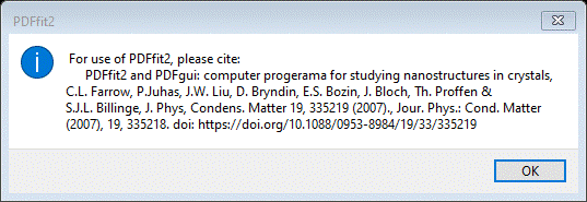
In this and subsequent tutorials, we will show how to use GSAS-II in conjunction with PDFfit2 (“PDFfit2 and PDFgui: computer programs for studying nanostructures in crystals", C.L. Farrow, P.Juhas, J.W. Liu, D. Bryndin, E.S. Bozin, J. Bloch, Th. Proffen & S.J.L. Billinge, J. Phys, Condens. Matter 19, 335219 (2007), Jour. Phys.: Cond. Matter (2007), 19, 335218. doi: https://doi.org/10.1088/0953-8984/19/33/335219) to fit pair distribution functions (PDF) with a “small box” disordered model. We will refer to PDFfit2 as “PDFfit” in this & subsequent tutorials as well as in the GSAS-II user interface for it.

The GSAS-II interface to PDFfit is a simplification where some capabilities of PDFfit are not implemented; GSAS-II only allows a single phase for PDFfit and the atom thermal displacement model is strictly isotropic. PDFfit allows multiple phases and anisotropic thermal motion; we considered these to be not useful and an unneeded complication, and these are better tackled via Rietveld refinement with the original diffraction data.

We have included with the GSAS-II distribution the most recent version of the PDFfit2 executable and its python interface routines for Windows (those for Mac OSX and linux will follow in due course). They are in the diffpy subdirectory of GSAS-II. No other files are needed. Also, the diffpy/manual subdirectory has the paper referenced above as well as one that described the original Fortran version of PDFfit. PDFgui.html describes 3 tutorials, upon which the GSAS-II ones are based, as given for the PDFgui software. Alternatively, you can install pdffit2 from Anaconda by executing

conda install -c diffpy diffpy.pdffit2

in a console window after activating your version of python. It will be installed in your python as gsas2full/Lib/site-packages/diffpy.

In this tutorial we will use a simple analysis for Ni using neutron G(r) and x-ray G(r) patterns to introduce you to the process of doing PDFfit analysis within GSAS-II. If you haven’t done so already, start GSAS-II.

Step 1. Setup parent Ni phase

The blank startup view of GSAS-II begins with this

Do Data/Add new phase and enter Ni to replace “New phase” in the popup. The window will be redrawn

Change the space group to F m 3 m (don’t forget the spaces). This will be done in a popup and a second popup will show the operators for Fm3m; the window will be redrawn to show the required entry for the unit cell. Enter 3.524 for Unit cell a; the window should show

Now select the Atoms tab; it will be empty

Do Edit Atoms/Append atom; a dummy atom will appear

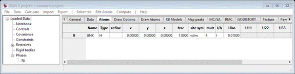
Double left-click on the atom type (“H”), after a short pause a popup with a periodic table will appear. Select Ni & press OK; the Atoms tab will be redrawn

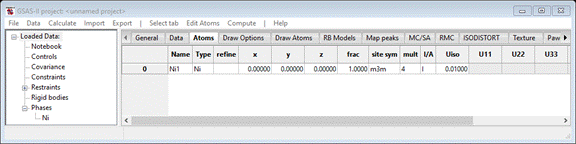
The nickel atom is already in the correct position (0,0,0) so we are done setting up the parent Ni phase.

Step 2. Make the PDFfit phase

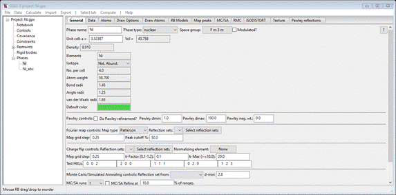
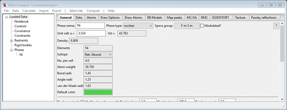
Because PDFfit utilizes no symmetry information from the space group that is associated with the structure to be studied, it requires a full unit cell of atom positions. This step uses the Transform tool in GSAS-II to generate these as a new phase. Return to the General tab for the Ni phase you should see

Do Compute/Transform; a popup will appear

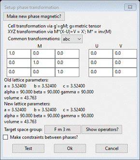
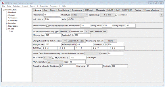
Change the Target space group to P 1 and press Ok. A new phase with the name “Ni abc” will appear; this will be used for the PDFfit analysis. The General tab for the new phase shows

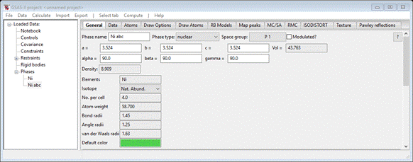
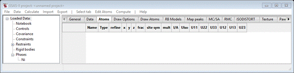
The phase name “Ni abc” is ok for the rest of GSAS-II, but unfortunately must be changed for PDFfit – it cannot contain any spaces, because it is used to create various file names and PDFfit is not able to handle file names with spaces. Change the phase name to “Ni_abc” (you can use anything else just so long as the name has no spaces & isn’t “Ni”). The Atoms tab shows 4 atoms as the unit cell contents.

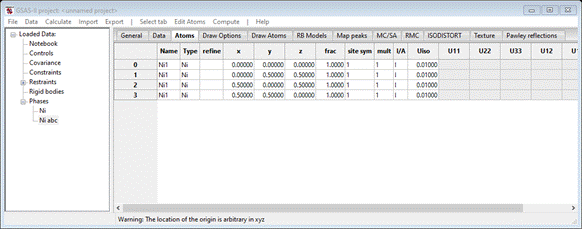
which is the correct full cell description for nickel suitable for use in PDFfit.

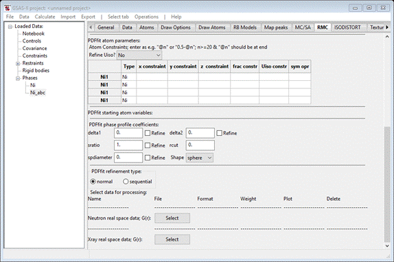
Step 3. Setup PDFfit

All operations for PDFfit are done in the RMC tab; select it and you should see the interface for the default (RMCProfile)

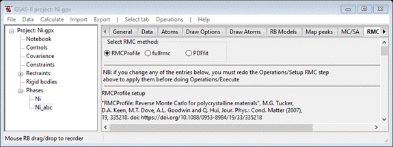
Select the radio button at the top for PDFfit; the window will be redrawn

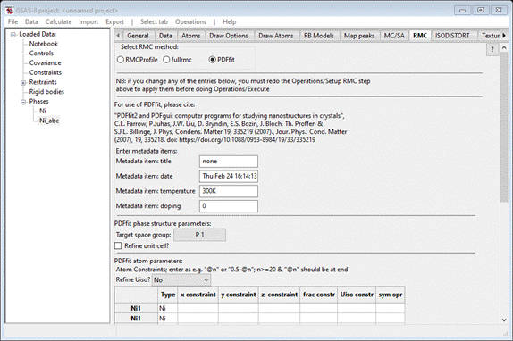
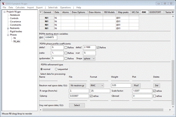
This is the top half of the PDFfit interface and one sees the setup is based on the Ni_abc phase (note the underscore you inserted in the phase name – this is essential for correct PDFfit operation). You may enter items in the metadata for your convenience; they play no role in the fitting by PDFfit. However, you must change the Target space group from P 1 to F m 3 m so that proper symmetry is used for lattice parameter refinement by PDFfit. Check the Refine unit cell box. Shifting to the lower part of the interface we see

You want to refine the Ni atom thermal motion parameters as a single value; select “by type” in the Refine Uiso? pulldown box. The window will be repainted showing “@81” for each of the Uiso constr items in the table. This symbolism is used for PDFfit variables; the code is “@N” where N is an integer. In GSAS-II we have assigned classes of variables their own set of integers; we will see these after we run PDFfit fo the first time.

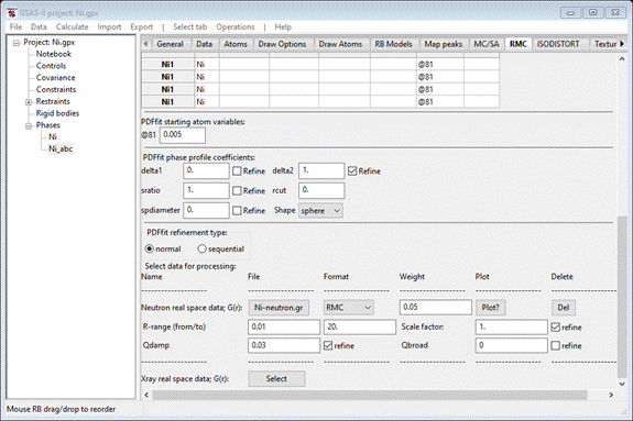
The coefficients “delt1” and “delt2” are for PDF sharpening effects due to atom-atom correlated motion. They depend on 1/r_ij and 1/r_ij², respectively. Similarly, “sratio” is a PDF sharpening for correlated motion of bonded atoms out to the distance limit “rcut” (not refinable). It is not likely that both descriptions will be used simultaneously (might lead to singularities in PDFfit!). The remaining term, “spdiameter” (Å), is a diameter for a nanoparticle sphere and is used for damping the calculated PDF at larger R. 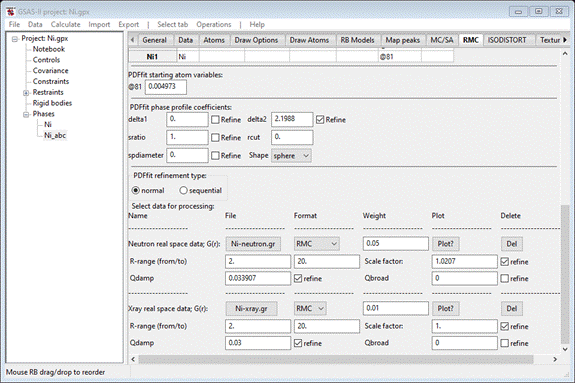If spdiameter = 0, this damping is not used. Here we will be refining only delta2, set it to 1.0 & check it’s refine box.

Next, press the “Neutron real space G(r)” Select button; you will first be asked to provide a GSAS-II project name (I used “Ni”) in a file dialog box. Next it will show another file dialog box. Navigate to PDFFIT-I/data and select “Ni-neutron.gr”. It opens this file and refreshes the RMC tab to show the new data set

If you press the Plot? button, a plot of Ni-neutron.gr will be shown

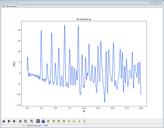
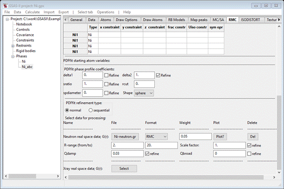
Note that the 1^st peak is at 2.45A; this is the nearest neighbor Ni-Ni distance. You will want to set the value in the R-range 1^st box to be a bit below that (I used 2.0). (NB: PDFfit will crash if this value is zero, so choose something suitable). The two PDF Gaussian broadening coefficients: “Qdamp” depends on the limiting Q range of the original diffraction data, and “Qbroad” depends on the noise level in the high Q diffraction data. If zero, they are not used. We should use Qdamp=0.03 as a starting value & refine it. The “scale factor” is nominally unity for PDF data but can differ due to e.g. absorption effects in the original data; thus it should be refined. When done the window should look like

This completes the initial setup for PDFfit. Save the project file.

Step 4. Running PDFfit

PDFfit executes by running in a separate process a short python script that contains parameter setup values, refinement codes, etc. This is prepared automatically by GSAS-II; do Operations/Setup RMC from the menu bar. A message will appear on the console and 2 new files will appear in your working directory. They will be named “Ni_abc-PDFfit” with different extensions (.py and .stru).

To run PDFfit, do Operations/Execute from the menu bar. You will first see a reminder to properly acknowledge your use of PDFfit (don’t forget to cite GSAS-II as well!).

Press OK. A new console window will appear and run very quickly. A banner for PDFfit appears followed by setup information and then its progress on refining the Ni structure. The end of the display has convergence information (R_w = 6.975%; a good fit) and a “Press any key to continue . . .” message.

Press any key, the console will vanish, and a new popup appears

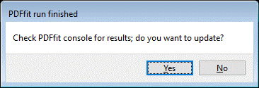
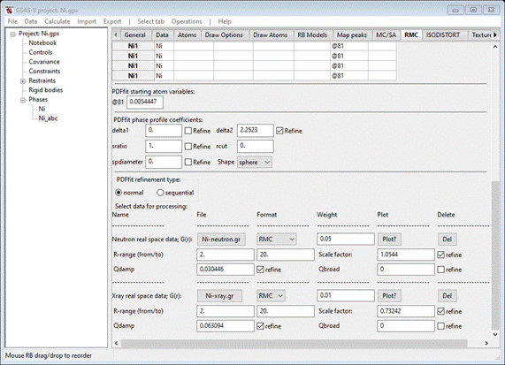
Press Yes, The RMC window is repainted with updated values and some additional information (in the lower part)

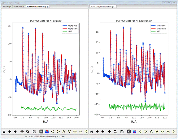
If you do Operations/Plot from the menu, a plot showing the fit will appear

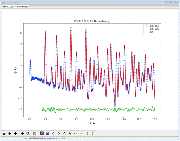
The blue curve is the original G(r) data, the red line is the fit and the green line is the difference. Your working directory will have 3 additional files all named “Ni_abc-PDFfit” with the extensions “res”, “rstr” and “fgr” (and an “N” in the latter file name). The first is a listing of the setup information and results from the last refinement cycle. Ni_abc-PDFfit.rstr is an updated version of the .stru fine and contains updated phase and atom results with esds. The .fgr file contains the observed and calculated PDF. Note that the lattice parameters in the General tab have been updated and the Uiso values for the Ni atoms are shown as anisotropic in the Atoms tab. Note that the “Plot?” button does not produce this plot with obs & calc curves; it is intended only as a data inspection tool.

Step 5. Doing a combined neutron/x-ray PDF fit with PDFfit (optional)

If you wish, you can add the available x-ray PDF to this project and use PDFfit to fit both with a common Ni structure.

At the bottom of the RMC tab for PDFfit, press the “Xray real space data” Select button. A file dialog will appear. Navigate to PDFfit-I/data and select Ni-xray.gr; the RMC tab will be redrawn. Set the same flags as you used for the neutron G(r) entry. When done the window should look like

Next, do Operations/Setup RMC and then do Operations/Execute. Again, the fit will proceed very quickly; the console will show

The R_w = 7.00% is very good. Press any key to get back to GSAS-II. After accepting the results, the RNC window will be redrawn showing (at the bottom) both data sets & their new parameters

Do Operations/Plot; two plots will appear. One is for the neutron data and the other for the x-ray data. For Ni they are virtually identical; I show them here side-by-side. This can be done in GSAS-II by dragging one plot tab to the right edge of the window; a light blue frame will appear to show the screen has been split. Release the mouse button. You can undo this by dragging the tab back to the main plot tab set.

If you examine the results file Ni_abc-PDFfit.res, you can find a short table near the end

Refinement parameters:

1: 1.05439 (0.013) 2: 0.0304455 (0.0026) 3: 0.732419 (0.00073)

4: 0.0630938 (0.00011) 10: 2.25235 (0.015) 11: 3.53157 (1.9e-05)

81: 0.00544471 (6.9e-06)

The values with esds are given for each refined parameter; the parameter numbers are those used in the “@N” symbolism used by PDFfit. These have been automatically assigned by GSAS-II according to the type of parameter to avoid unintended conflicts. The first two are scale & Qdamp for the neutron data set and the next two are those for the x-ray data set. Numbers 1-9 are reserved for these types of data parameters. #10 is for the delta2 phase parameter and #11 is the Ni lattice parameter. Numbers 10-19 are reserved for phase & lattice parameters. Although none are used in this example, atom coordinates use parameter numbers in the range 20-79. Finally, #81 is the Ni Uiso term: thermal motion parameter numbers are 81 or greater. The next tutorial will give more complex uses of these parameter codes.

This completes this introductory tutorial for PDFfit in GSAS-II; you can save your project if you wish.