Magnetic Structures in GSAS-II - Tutorial V

Exercise files are found here

Introduction

In this tutorial, we will show how GSAS-II makes use of the Bilbao crystallographic server (www.cryst.ehu.es/) Magnetic Symmetry and Applications routine k-SUBGROUPSMAG (Perez-Mato, JM; Gallego, SV; Elcoro, L; Tasci, E and Aroyo, MI, J. of Phys.: Condens Matter (2016), 28:28601) to determine a magnetic crystal structure with two non-zero propagation vectors. If you have not done so already, you may wish to do the Simple Magnetic Structures tutorial first as it contains some background information that will not be covered here. It is also helpful to do parts I - IV of the series of Magnetic Structures tutorials. To make this work, your computer must have an internet connection for GSAS-II to access this site. (We will supply the project file that results after k-SUBGROUPSMAG is called in case you lack internet access).

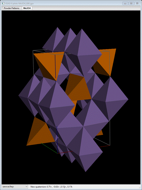
In this tutorial we will be examining Mn₃O₄ (hausmannite), which shows two apparent magnetic phase transitions between the paramagnetic phase above T_N = 41K and the lowest temperature explored (4.7K). The paramagnetic phase of Mn₃O₄ is a tetragonal distortion of the cubic spinel structure (drawing above) with space group I4₁/amd, a=5.765 and c=9.442 Å at room temperature. Time-of-flight (TOF) neutron powder diffraction data of the paramagnetic phase was collected on POWGEN (SNS, Oak Ridge National Laboratory) at 60K and the magnetic phase at 10K with 2 frames of data for each. The magnetic structure was originally determined by Boucher, et al. (Boucher, B., Buhl, R. & Perrin, M. (1971), J. Phys. Chem. Solids, 32, 2429-2437) and reexamined by Jensen & Nielsen (Jensen, J.B. & Nielsen, O.V. J. Phys. C: Solid State Phys. (1974), 7, 409-424). We will first refine the paramagnetic phase and use that as the starting point for the magnetic structure determination. As we will see the magnetic space group is a subgroup of I4₁/amd by both a loss the body centering symmetry and a unit cell doubling along one of the equivalent tetragonal a,b-axes. We will use k-SUBGROUPSMAG to help sort this out. NB: the Bilboa MAGNDATA data base contains an entry for Mn₃O₄ (#1.1), but it is for a different phase of this material and is thus unrelated to this tutorial.

If you have not done so already, start GSAS-II (make sure about the internet connection!).

Refinement of paramagnetic Mn₃O₄

Step 1. Read in the data files

1. Use the Import/Powder Data/from TOPAS xye or Fit2D chi file menu item to read the data file into the current GSAS-II project. This read option is set to read the xye format (angles in degrees) used by Topas, etc. Because you used the Help/Download tutorial menu entry to open this page and downloaded the exercise files (recommended), then the Magnetic-V/data/... entry will bring you to the location where the files have been downloaded. (It is also possible to download them manually from https://subversion.xray.aps.anl.gov/pyGSAS/Tutorials/Magnetic-V/data/. In this case you will need to navigate to the download location manually.)
For this tutorial you will see the data file in the file browser, because the extensions on data files are the expected ones.

2. Select the PG3_20256-2_60K.xye data file in the first dialog and press Open. There will be a Dialog box asking Is this the file you want? Press Yes button to proceed. NB: Don’t be tempted to read both data sets at once. The problem with the xye format is that it has no provision for identifying the instrument parameter file or the frame (“Bank”) number of the data. If you did read both, then GSAS-II would use the instprm file read in the next step and apply it inappropriately to both data sets. One can recover from this error by selecting Instrument parameters and doing Operations/Load parameters with the correct file. Since this data file does not define an instrument parameter file, a file dialog will appear for you to select the correct instrument parameter file. Select Bank 2.instprm; you may have to change the file type in the file selection Dialog box to GSAS-II instprm file to see it. At this point the GSAS-II data tree window will have several entries

and the plot window will show the powder pattern

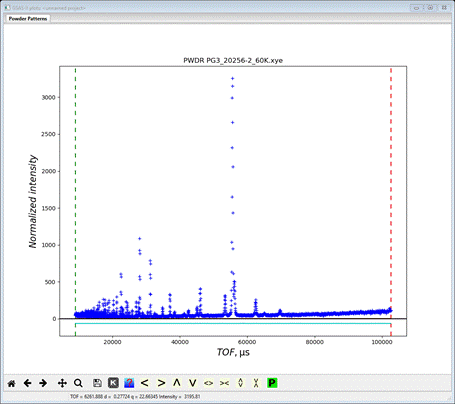
which covers the d-spacing range 0.4-4.545 Å. This is the high resolution frame for POWGEN and is collected by a selected setting of the beam choppers. Go to Limits

We want to remove the uninteresting high TOF part and limit the low TOF to something reasonable. I used 12500 and 75000; the lower one corresponds to d_min~0.55 Å and the upper one is just beyond the last visible peak. Now we have to read the other frame.

3. Do Import/Powder Data/from TOPAS xye or Fit2D chi file and select the PG3_20269-4_60K.xye data file in the first dialog and press Open. There will be a Dialog box asking Is this the file you want? Press Yes button to proceed.

4. Since this data file does not define an instrument parameter file, a file dialog will appear for you to select the correct instrument parameter file. Select Bank 4.instprm; you may have to change the file type in the file selection Dialog box to GSAS-II instprm file to see it. At this point the GSAS-II data tree window will have more entries

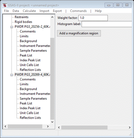
And the plot will show this larger d-spacing (1.15-9.0 Å) frame collected with a different set of chopper settings. Notice that there is now a peak (d=4.94 Å) which was beyond the range of the other frame. Go to Limits for this data set and set the upper limit to 125000; leave the lower limit as it is.

Step 2. Read in the chemical structure for Mn₃O₄ (hausmannite)

1. Use the Import/Phase/from CIF file menu item to read the phase information for Mn₃O₄ into the current GSAS-II project. This read option is set to read Crystallographic Information Files (CIF). Other submenu items will read phase information in other formats. Because you used the Help/Download tutorial menu entry to open this page and downloaded the exercise files (recommended), then the Magnetic-V/data/... entry will bring you to the location where the files have been downloaded. (It is also possible to download them manually from https://subversion.xray.aps.anl.gov/pyGSAS/Tutorials/Magnetic-V/data/. In this case you will need to navigate to the download location manually.)

2. Select the Mn3O4-Hausmannite.cif data file in the first dialog and press Open. There will be a Dialog box asking Is this the file you want? Press Yes button to proceed. You will get the opportunity to change the phase name next (I took out the space!); press OK to continue.

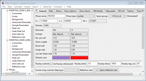
Next is the histogram selection window; this connects the phase to the data so it can be used in subsequent calculations. Select the histograms (or press Set All) and press OK. The General tab for the phase is shown next

Step 3. Structure refinement

We are now ready for initial refinement of scale and background. Do Calculate/Refine from the main menu; a File Selection dialog will appear wanting a file name for your project. I used Mn3O4 60K; the refinement proceeded quickly. The fit is ok for a start (wR ~23%), mostly from poorly fitting background; select Background for both PWDR data sets and change the number of terms to 6. Then go to the Mn3O4 phase and set the lattice parameter refinement. Do Calculate/Refine; the residual will be much improved (wR=13.4%). Finally, go to the Atoms tab and set refinement flags XU for all atoms. Do Calculate/Refine; the residual will be a bit better (wR = 10.16%). This is a pretty good fit; we should be able to get as good a fit with the magnetic structure. We are done with this step; Save the project & close GSAS-II; we will use this phase information for the magnetic structure study.

The magnetic structure of Mn₃O₄ at 10K

Step 1. Read in the data files

If you have not done so already, start GSAS-II (make sure about the internet connection!).

2. Select the PG3_20254-2_10K.xye data file in the first dialog and press Open. There will be a Dialog box asking Is this the file you want? Press Yes button to proceed. NB: Don’t be tempted to read both data sets at once. The problem with the xye format is that it has no provision for identifying the instrument parameter file or the frame (“Bank”) number of the data. If you did read both, then GSAS-II would use the instprm file read in the next step and apply it inappropriately to both data sets. One can recover from this error by selecting Instrument parameters and doing Operations/Load parameters with the correct file.

3. Since this data file does not define an instrument parameter file, a file dialog will appear for you to select the correct instrument parameter file. Select Bank 2.instprm; you may have to change the file type in the file selection Dialog box to GSAS-II instprm file to see it. At this point the GSAS-II data tree window will have several entries

and the plot window will show the powder pattern

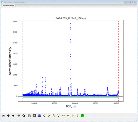
which covers the d-spacing range 0.4-4.545 Å. This is the high resolution frame for POWGEN and is collected by a selected setting of the beam choppers. Go to Limits

We want to remove the partial peak at high TOF and limit the low TOF to something reasonable. I used 12500 and 100000; the lower one corresponds to d_min~0.55 Å and the upper one is just excludes the last visible peak. Now we have to read the other frame.

4. Do Import/Powder Data/from TOPAS xye or Fit2D chi file and select the PG3_20255-4_10K.xye data file in the first dialog and press Open. There will be a Dialog box asking Is this the file you want? Press Yes button to proceed.

5. Since this data file does not define an instrument parameter file, a file dialog will appear for you to select the correct instrument parameter file. Select Bank 4.instprm; you may have to change the file type in the file selection Dialog box to GSAS-II instprm file to see it. At this point the GSAS-II data tree window will have more entries

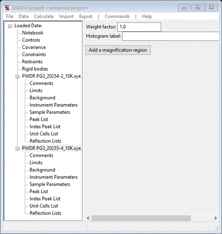
And the plot will show this larger d-spacing (1.15-9.0 Å) frame collected with a different set of chopper settings. Notice that there is now a peak (d=4.94 Å) which was beyond the range of the other frame. Go to Limits for this data set and set the upper limit to 125000; leave the lower limit as it is.

Step 2. Read in the chemical structure for Mn₃O₄ at 60K

1. Use the Import/Phase/from GSAS-II gpx file menu item to read the phase information for Mn₃O₄ into the current GSAS-II project. The file you want is the one from the 1^st part of this tutorial and should be in your current directory. This read option is set to read from other GSAS-II project files. Other submenu items can read phase information in other formats.

2. Select the Mn3O4 60K.gpx data file in the first dialog and press Open. There will be a Dialog box asking Is this the file you want? Press Yes button to proceed. You will get the opportunity to change the phase name next; press OK to continue.

Step 3. Check powder pattern indexing

Here the objective is to determine how the reflection positions generated from the chemical (“nuclear”) crystal structure lattice match up with the peaks observed for this magnetic phase.

1. Select Unit Cells List from the tree entries under the 2^nd histogram (PWDR PG3_20255-4_10k.xye & has the largest d-spacing peaks); the Indexing controls will be shown

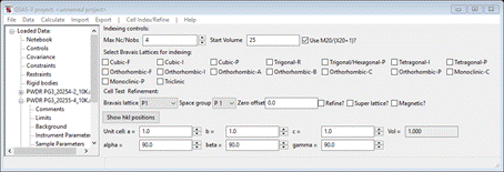
This can be use lattice parameters & space groups to generate expected reflection positions to check against the peaks in the powder pattern.

One could then enter Bravais lattice, choose space group & enter lattice parameters by hand, but the easy way is to use the chemical lattice directly. Do "Cell Index/Refine"/"Load Phase" from the menu; since there is only one phase available, it is selected, but if more that one were present a Phase selection box would appear to offer a choice. Note that the "Import Cell" menu item allows you to get lattice information from a phase in a file (which can be in any of the formats that GSAS-II can read). The Indexing controls will change, as shown:

This shows the symmetry settings and lattice constants for Mn₃O₄ you had obtained from the gpx file and the powder pattern will change showing the lines for I 41/amd and the Mn₃O₄ lattice parameters. Change the space group to I 4/m m m; the plot will change showing the new lines allowed with body centering, but no other extinction conditions.

Notice that some lines are not indexed; perhaps we need to double one of the axes to generate reflections for these. Add “*2” at the end of the a-axis; this will index some lines but remove it from others. Try doing the same for the c-axis; doesn’t appear to help either. Bring both back to the original values (add “/2” as needed to each, or else just do Load Phase again). Recall that the chemical unit cell is I-centered; maybe the centering is lost in forming the magnetic space group. Set the Bravais lattice to P4/mmm and the space group to match. Then try doubling the a-axis; that indexes every line. So, we need two parts to the propagation vector; one to double a (or b) and one to remove the centering. This makes sense considering the report that there are two low temperature phase transitions for this material. They would be (1/2,0,0) or (0,1/2,0) and (0,0,0). Of the first two, I’m going to pick (0,1/2,0) for the 1^st one as that will match what was originally used.

Step 4. Run k-SUBGROUPSMAG

In this next step, you will be accessing the Bilbao crystallographic server so you must be connected to the internet. First, reset to the initial I41/amd symmetry and cell parameters for the Mn3O4 phase, which can be done easily reusing the "Cell Index/Refine"/"Load Phase" menu item again. Then, in the "Cell Index/Refine" menu select "Run k-SUBGROUPSMAG"; a small popup dialog will appear

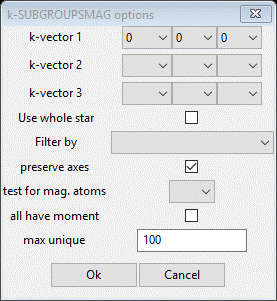
To set the propagation vectors to (0,1/2,0) and (0,0,0), set y for k-vector 1 to 1/2 and x, y & z for k-vector 2 to 0, 0, 0 (NB: don’t leave any blank – not the same as zero; k-SUBGROUPSMAG will fail if you do). Select Mn for the mag atoms test and check the last box so we see solutions with all magnetic Mn atoms marked as “Keep”. Press Ok; a popup dialog will appear reminding you how to cite the Bilbao routine in any paper you write using this facility.

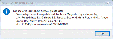
Press Ok, the nag note will also appear on the console and after a pause, the console will show “request OK” indicating that the Bilbao site has responded with some results. GSAS-II will next display a File Dialog asking for a project name to save this project; change the directory to a useful place for your work on this tutorial and give the project a name; I used Mn3O4 10K.

The GSAS-II data window will display the 205(!) results from k-SUBGROUPSMAG. (If k-SUBGROUPSMAG failed because you lack internet access, this file is located in the same location as the powder data and cif files used above were found. Do File/Open Project from the main menu to access it as “Mn3O4 10K.gpx”, then do Save as to save it immediately in your working directory.).

The Unit Cells List window will show the results

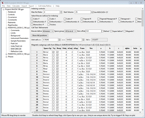
There are a lot of possible solutions; the lowest number of unique positions is 4. Let’s change the filters to Keep only those. Double click the Keep column heading; a popup will appear

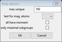
Set max unique to 4, the test for mag atoms to Mn, the all have moment box and press OK. That cleared away a lot of solutions

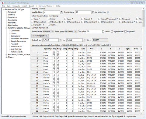
In fact there are only 4 left from the initial 205 possible space groups; we’ll have to look at each in turn. If you do Try on each, unfortunately there are no reflections within our TOF frames that systematically change so we can discriminate between them. If you then click on the number in the Uniq column (4 in each case), GSAS-II will show the unique magnetic atom positions and their magnetic moment components. For #2 (Pbn’a’) we see

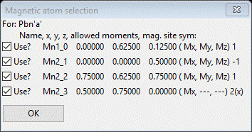
Press OK & try the next one (#3 Pb’n’a)

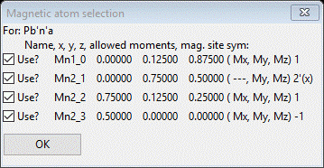
Again press OK & try the next (#4 Pb’na’)

Press OK and finally the last one (#8 Pbna)

These seem to be in pairs two (#2 & #8) with no My, Mz component on one atom and the other two (#3 & #4) with no Mx component on one atom; the other atoms are in general positions and have all three components allowed. One other point for consideration is that the Mn oxidation states are in the + 2 to +4 range so the high spin magnetic moments could be large (4-5m_B). We will still have to try each in turn. Before we start we should go to the Mn3O4 phase, clear the Unit cell refine flag and then select Atoms and clear the refine flags there; this will avoid problems for our first refinements. Save the project.

Step 5. Trial magnetic structures for Mn₃O₄

Intoduction

In this section we will be doing the same thing using each of the 4 possible magnetic solutions with the minimum number (4) of magnetic atoms. For each one we have opened the initial one phase project containing the k-SUBGROUPSMAG table of possible magnetic space groups. We then select one, assign values to the magnetic components and then do sufficient refinements to be able to compare them.

1. Try Pbn’a’ (#2)

To begin, be sure Mn3O4 10K.gpx is opened in your GSAS-II. Select the Mn3O4 phase and do Compute/Select magnetic/subgroup phase; a popup selection will appear

Select the 1^st one and press OK; a new popup will appear

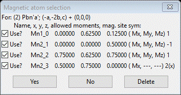
Press Yes; a new project will be created Mn3O4 mag_2.gpx and you will be at the General tab for the new magnetic phase

Select Atoms and enter 2.0 for every Mx My Mz allowed for all 4 atoms; it should look like

Do Calculate/Refine for Scale & Background for 2 data sets (wR = 27.6%). Set refine for all Mn atoms to M and do Calculate/Refine 2-3 times to convergence (wR=20.6%).

Next select the General tab for each phase and check the Refine unit cell box for each. Now do Calculate/Refine until convergence (my wR=16.4% after several refinements).

Save the project; we may look at it later for more refinement.

2. Try Pb’n’a (#3)

To begin, be sure Mn3O4 10K.gpx is opened in your GSAS-II; we are going to repeat the above steps. Select the Mn3O4 phase and do Compute/Select magnetic/subgroup phase; a popup selection will appear

We’ve done the 1^st one; now pick the 2^nd and press OK. A new popup will appear

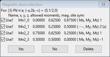
Press Yes; a new project will be created Mn3O4 mag_3.gpx and you will be at the General tab for the new magnetic phase

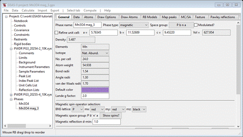
Select Atoms and enter 2 for every Mx My Mz allowed for all 4 atoms; it should look like

Do Calculate/Refine for Scale & Background for 2 data sets (wR = 25.1%). Set refine for all Mn atoms to M and do Calculate/Refine 2-3 times to convergence (wR=20.9%).

Next select the General tab for each phase and check the Refine unit cell box for each. Now do Calculate/Refine until convergence (my wR=16.9% after several refinements).

Save the project; we may look at it later for more refinement.

3. Try Pb’na’ (#4)

We’ve done the 1^st two; now pick the 3rd and press OK. A new popup will appear

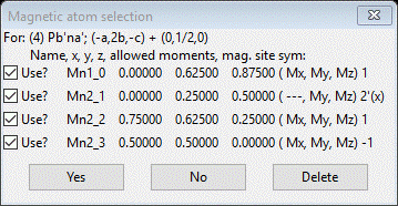
Press Yes; a new project will be created Mn3O4 mag_4.gpx and you will be at the General tab for the new magnetic phase

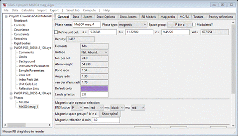
Select Atoms and enter 2 for every Mx My Mz allowed for all 4 atoms; it should look like

Do Calculate/Refine for Scale & Background for 2 data sets (wR = 25.9%). Set refine for all Mn atoms to M and do Calculate/Refine 2-3 times to convergence (wR=19.9%).

Next select the General tab for each phase and check the Refine unit cell box for each. Now do Calculate/Refine until convergence (my wR=15.8% after several refinements).

Save the project; we may look at it later for more refinement.

4. Try Pbna (#8)

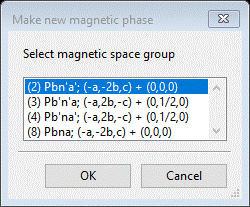
We’ve done the 1^st three; now pick the last one (#8) and press OK. A new popup will appear

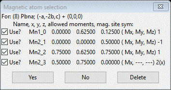
Press Yes; a new project will be created Mn3O4 mag_4.gpx and you will be at the General tab for the new magnetic phase

Select Atoms and enter 2 for every Mx My Mz allowed for all 4 atoms; it should look like

Do Calculate/Refine for Scale & Background for 2 data sets (wR = 28.8%). Set refine for all Mn atoms to M and do Calculate/Refine 2-3 times to convergence (wR=22.7%).

Next select the General tab for each phase and check the Refine unit cell box for each. Now do Calculate/Refine until convergence (my wR=19.4% after several refinements).

Save the project; we may look at it later for more refinement.

Review results and complete refinement

Comparing the final wR values for the 4 structures gives the following order: 1) Pb’na’ (#4) wR=15.8%, 2) Pbn’a’ (#2) wR= 16.4%, 3) Pb’n’a (#3) wR=16.9% and 4) Pbna (#8) wR=19.4%. Clearly, #8 is poorest and #4 is best in terms of residuals. The pattern for the higher d-spacing frame shows the fit

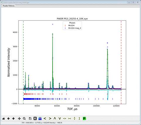
The principal problem seems to be peak positions; the magnitudes seem ok which indicates that the magnetic structure is correct.

Looking at the magnetic moment components, it appears that Mx could be zero for all atoms. Let’s try this; set all Mx = 0. Now we have to add holds on these in Constraints to keep them at zero (and avoid possible least-squares singularities). Go to Constraints and do Edit Constr./Add hold; a popup will appear

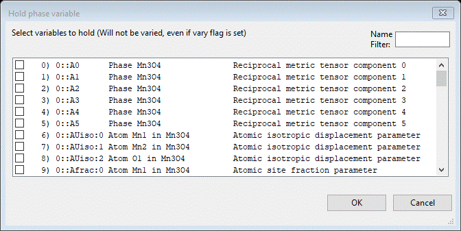
Use Mx for the filter and select all that shows (it doesn’t matter that one is fixed by symmetry). The Constraints list will show the holds at the bottom

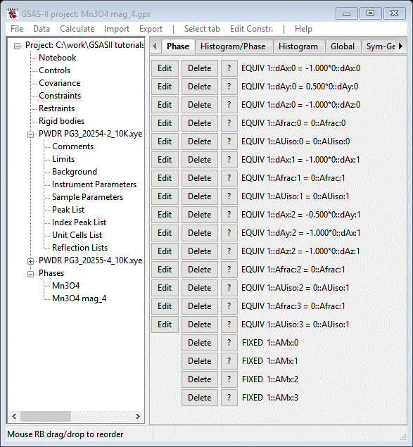
Do Calculate/Refine until convergence (wR=15.8%); it is essentially unchanged showing that Mx=0 is a valid assumption. In addition it appears that Mz=0 for the 1^st Mn atom. Set Mz=0 for it and add the appropriate hold for it to the constraints list. Finally we can refine the remaining atom parameters; set U for all atoms and XU for the O-atom in the chemical cell, and UM for all Mn atoms in the magnetic cell. Whatever constraints are needed to tie these together have already been entered in the Constraints list. Do Calculate/Refine until convergence (wR=15.9%); the residual is essentially unchanged. These parameters were already well determined from the 60K data. We still see peak position errors especially for the magnetic peaks at high d-spacing. This probably arises from a bit of magnetically induced strain on the lattice. We can explore this by refining the Dij coefficients for the magnetic phase. Go to the Data tab for the magnetic phase

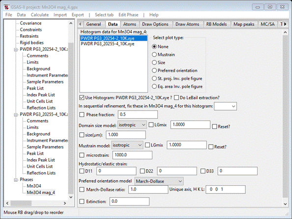
and set the refine boxes for D11 D22 & D33 for both histograms. (do not be tempted to do the same for the chemical phase – that will result in a singular matrix error because of the coupling with the lattice parameters). Do Calculate/Refine until convergence; my wR=15.2% is significantly better showing that magnetic strain is a possibility. Since D11 & D33 are < than D22, they could be reset to zero & not refined. In that case wR=15.2% again indicating that all the magnetic strain is along the b-axis (the one that was doubled). This analysis is not strictly correct because it does not allow the chemical cell to show the magnetic strain. To do this one has to describe the chemical structure in the doubled magnetic cell with the space group Pbna (probably doubling or more the number of atom positions and having a very unstable refinement to deal with). Next we examine our result.

Go to the Draw Atoms tab for the magnetic phase. Then select all the atoms and do Edit Figure/Fill unit cell. The structure will be redrawn showing the complex magnetic structure.

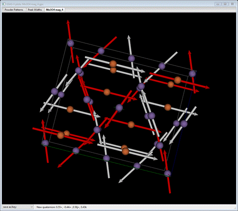
I’ve colored the tetrahedral Mn atoms as orange to distinguish them from the octahedral ones; you can do that by selecting Mn1_0 from the Name column (double click the heading and select from the popup). Then do Edit Figure/Atom color; select the color from the palette. The tetrahedral ones are ordered aligned ferromagnetically along the doubled b-axis while the rest are in two intersecting ferromagnetic layers to give an overall antiferromagnetic structure. This arrangement is essentially that of Jensen & Nielsen but with a properly selected magnetic space group, Pb’na’, as a subgroup of I4₁/amd, and associated set of unique magnetic Mn atoms. This completes this tutorial, you can save the project if you wish.

Magnetic Structures in GSAS-II - Tutorial V

Introduction

Refinement of paramagnetic Mn3O4

Step 1. Read in the data files

Step 2. Read in the chemical structure for Mn3O4 (hausmannite)

Step 3. Structure refinement

The magnetic structure of Mn3O4 at 10K

Step 1. Read in the data files

Step 2. Read in the chemical structure for Mn3O4 at 60K

Step 3. Check powder pattern indexing

Step 4. Run k-SUBGROUPSMAG

Step 5. Trial magnetic structures for Mn3O4

Intoduction

1. Try Pbn’a’ (#2)

2. Try Pb’n’a (#3)

3. Try Pb’na’ (#4)

4. Try Pbna (#8)

Review results and complete refinement

Refinement of paramagnetic Mn₃O₄

Step 2. Read in the chemical structure for Mn₃O₄ (hausmannite)

The magnetic structure of Mn₃O₄ at 10K

Step 2. Read in the chemical structure for Mn₃O₄ at 60K

Step 5. Trial magnetic structures for Mn₃O₄