Magnetic Structures in GSAS-II - Tutorial IV
Introduction
In this tutorial, we will show how GSAS-II makes use of the Bilbao crystallographic server (www.cryst.ehu.es/) Magnetic Symmetry and Applications routine k-SUBGROUPSMAG (Perez-Mato, JM; Gallego, SV; Elcoro, L; Tasci, E and Aroyo, MI, J. of Phys.: Condens Matter (2016), 28:28601) to determine a magnetic crystal structure with a non-zero propagation vector. If you have not done so already, you may wish to do the Simple Magnetic Structures tutorial first as it contains some background information that will not be covered here. It is also helpful to do parts I - III of the series of Magnetic Structures tutorials. To make this work, your computer must have an internet connection for GSAS-II to access this site. (We will supply the project file that results after k-SUBGROUPSMAG is called in case you lack internet access).
Note that to access the Bilboa Crystallographic Server from inside GSAS-II you must register for access. This only needs to be done once. See the Setup Access to the Bilbao Crystallographic Server tutorial for details on how to do this.

In this tutorial we will be examining the perovskite (Pr0.5Sr0.5)MnO3, which at low temperature is a doubled a,b,c-axis variant due to a rotation of the MnO6 octahedra about the assigned c-axis (drawing above) to give the Fmmm, a=7.508, b=7.812, c=7.684 Å chemical unit cell. The neutron powder diffraction data was collected on the 3T2 diffractometer (LLB, Saclay France) at 10K and λ=1.227 Å and this tutorial is based on Example 12.3 in the Jana2006 Cookbook (Dušek, et al., 2017). The antiferromagnetic structure was originally determined by Knížek, et al. (K. Knížek, J. Hejtmánek, and Z. Jirák, C. Martin, M. Hervieu, and B. Raveau, G. André and F. Bourée, Chemistry of Materials, (2004), 16, 1104-1110). As we will see the magnetic space group is a subgroup of Fmmm made principally by a loss of some of the face centering symmetry. We will use k-SUBGROUPSMAG to help sort this out.
If you have not done so already, start GSAS-II (make sure about the internet connection!).
Step 1. Read in the data file
1. Use
the Import/Powder Data/from gsas powder data
file menu item to read the data file into the current GSAS-II
project. Because you used the Help/Download tutorial
menu entry to open this page and downloaded the exercise files (recommended),
then the Magnetic-IV/data/...
entry will bring you to the location where the files have been downloaded. (It
is also possible to download them manually from https://advancedphotonsource.github.io/GSAS-II-tutorials/Magnetic-IV/data/.
In this case you will need to navigate to the download location manually.)
For this tutorial the extension on the data file is the expected one, so it
should be immediately visible.
2. Select the PrSrMnO.gda data file in the first dialog and press Open. There will be a Dialog box asking Is this the file you want? Press Yes button to proceed.
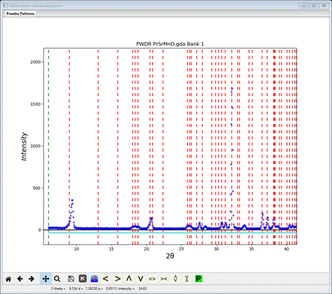
3. Since this data file does not define an instrument parameter file, a file dialog will appear for you to select the correct instrument parameter file. Select Saclay 3T2. instprm; you may have to change the file type in the file selection Dialog box to GSAS-II instparm file to see it. At this point the GSAS-II data tree window will have several entries and the plot window will show the powder pattern
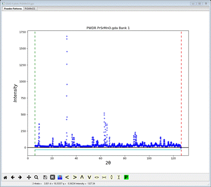
4. The last few points in the profile are problematic; I set the upper Limit to 123.5 to avoid them.
Step 2. Read in the chemical structure for (Pr.5Sr.5)MnO3
1. Use the Import/Phase/from CIF file menu item to read the phase information for (Pr.5Sr.5)MnO3 into the current GSAS-II project. The file you want is PrSrMnO.cif and should be in your current directory. Other submenu items can read phase information in other formats.
2. Select the PrSrMnO.cif data file in the first dialog and press Open. There will be a Dialog box asking Is this the file you want? Press Yes button to proceed. You will get the opportunity to change the phase name next (I changed it to PrSrMnO3); press OK to continue.
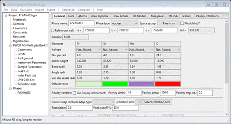
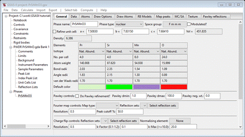
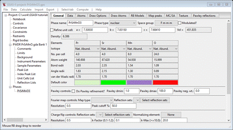
5. Next is the histogram selection window; this connects the phase to the data so it can be used in subsequent calculations. Select the histogram (or press Set All) and press OK. The General tab for the phase is shown next
Step 3. Check powder pattern indexing
Here the objective is to determine how the reflection positions generated from the chemical (“nuclear”) crystal structure lattice match up with the peaks observed for this antiferromagnet.
Select Unit Cells List from the tree entries under the
histogram (begins with PWDR); the Indexing controls will be shown

This can use lattice parameters & space groups to
generate expected reflection positions to check against the peaks in the powder
pattern. One could then enter this information by hand, but the easy way is to
use the chemical lattice directly. Do Cell
Index/Refine/Load Cell from the menu; a Phase selection box will
appear with only one choice (PrSrMnO3).
This was taken from the Phases present in this project; there could be more
than one depending on what you loaded/created earlier. The Import
menu item allows you to get lattice information from any one of the other phase
containing files known to GSAS-II. Press OK
and the Indexing controls will be change
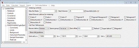
showing the lattice constants for (Pr.5Sr.5)MnO3 you had obtained from the cif file and the powder pattern will change showing the lines for Fmmm and those lattice parameters.
I’ve zoomed into the 6-40 deg range to see that a number of peaks are not indexed by this space group (NB: Fmmm lacks space group extinctions apart from F-centering so there is no need to change it as in previous tutorials) and lattice. As noted in the previous tutorial, antiferromagnetic ordering may force an increase in the unit cell dimensions (usually a doubling or tripling of one or more cell dimensions) or by removing a space group centering. Here we are starting with an F-centered chemical cell so a loss of centering to get either A-, B- or C- centering is a possibility to consider. To explore this we will try each in turn and see how the generated reflection positions match up with the observed peaks.
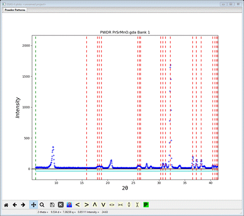
Change the Bravais lattice to Ammm and the Space group to A m m m; the plot will change on each choice to give

Those line up pretty well; note the lowest angle peak & the one at about 21º2Θ. Now change Bravais lattice and Space group to Bmmm; a new plot will appear
The match is not quite as good; the 1st line just misses the 1st peak top and the one at 21º2Θ also misses the peak top. Lastly, let’s try Cmmm; enter it for Bravais lattice and space group. A new plot appears

This fit seems even worse, so the right description is lose the B- and C-centering leaving just A-centering. However, we want the A-center to be magnetic; the way to do this is to assign the propagation vector kx,ky,kz = (1,0,0) when we run k-SUBGROUPSMAG on the parent space group (Fmmm).
Step 4. Run k-SUBGROUPSMAG
In this next step, you will be accessing the Bilbao crystallographic server so you must be connected to the internet. In the Cell Index/Refine menu select Run k-SUBGROUPSMAG; a small popup dialog will appear
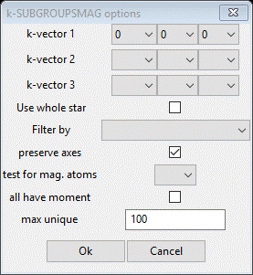
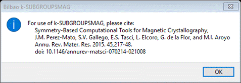
These are the controls for running the Bilbao routine. The space group (Fmmm) is taken from the Space Group entry on the Unit Cells window. Since we just discovered the propagation vector as (1,0,0) change kx1 to 1. The available selections were determined by surveying the known magnetic crystal structures given in the Bilbao Magnetic Structures database. Select Mn for the test for mag atoms and then press OK. A popup dialog will appear reminding you how to cite the Bilbao routine in any paper you write using this facility.
Press Ok,
the nag note will also appear on the console and after a pause, the console
will show “request OK” indicating that the Bilbao site has responded with some
results. GSAS-II will next display a File Dialog asking for a project name to
save this project; change the directory to a useful place for your work on this
tutorial and give the project a name; I used PrSrMnO3.
The GSAS-II data window will display the results from k-SUBGROUPSMAG. (If k-SUBGROUPSMAG failed because you lack internet access, this file is located in the same location as the powder data and cif files used above were found. Do File/Open Project from the main menu to access it as “PrSrMnO3.gpx”, then do Save as to save it immediately in your working directory.). The Unit Cells List window will show the results

The Uniq column gives the number of unique magnetic Mn atoms there are in each phase; usually the correct magnetic structure has the smallest number of these. The preserve axes option on the k-SUBGROUPSMAG is set by default to transform the standard setting result from k-SUBGROUPSMAG for orthorhombic to one that closely is aligned, if possible, to the parent cell axes. So this list contains non-standard settings of orthorhombic space groups (e.g. the chemical version of #3 PC bmn is a non-standard version of P mna, #53 in International Tables for Crystallography Vol A.). If desired, clearing the flag and rerunning k-SUBGROUPSMAG will produce magnetic space groups in standard settings; we will continue with the above set so the chemical cell and magnetic cell axes line up together.
Use the Try on the 4 marked Keep out of the 1st 8 solutions. Only #7 & #8 will index the low angle peaks correctly. We’ll go with these. The solutions further down are ones in which more than one symmetry generator was removed (nSup > 1); if need be we can go back and look at those. NB: running k-SUBGROUPSMAG with the “Landau transition” checked will give just these 1st 8 solutions. This might be appropriate because the magnetic transition for (Pr.5Sr.5)MnO3 is a continuous 2nd order transition. However, by doing this in other cases one might not see the correct result!
Step 5. Select 1st magnetic structure
Select the PrSrMnO3 phase from the GSAS-II data tree (under Phases). The General tab is shown for this nuclear phase.
Do Compute/Select magnetic phase; that will make a small popup dialog
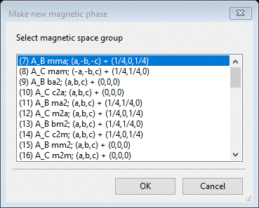
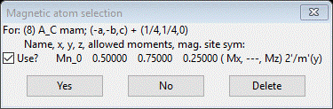
This shows all magnetic phases that were marked Keep in the Unit Cells List; for each you see the transformation and vector (the first two results we had checked to see if they indexed the pattern). Select the 1st one and press OK; a new popup dialog will appear.
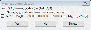
This one Mn atom has an allowed moment component (My). Press Yes to use it. The project will be saved first, then a file dialog box will appear offering a project name for this magnetic structure. It is named with the number from the space group list (PrSrMnO3 mag_7.gpx); press Save. The new project will be opened to the General tab for the AB mma magnetic phase just created.

Select Atoms, enter 1.0 for the Mn atom My values. Then go to Draw Atoms, select them all and do Edit Figure/Fill unit cell; you’ll see this antiferromagnetic structure

Do Calculate/Refine; the resulting wR ~26% with some intensity for all the peaks in the pattern, but the magnetic moment is probably wrong. Go to the magnetic phase Atoms tab and select refine M for the Mn atom. Do Calculate/Refine again; the residual drops a bit but now the errors seem to be mostly peak position. Go to the General tab for both phases and check the Refine unit cell box for each. Then go to Sample parameters for the PWDR data set, set goniometer radius to 1000 and check both Sample X & Y displ parameters. Do Calculate/Refine again; wR ~ 7% now. To finish the refinement, include Instrument parameters U, V, W, X, Y and SH/L; use 6 Background term and refine XU for all atoms in the chemical phase and XUM in the magnetic phase. After 2-3 sets of Calculate/Refine my residual was wR=6.15% and the magnetic Mn atom moment Mz = 3.41. The fit shown on the plot is quite good.
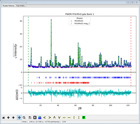
I show the plot with sqrt(intensity) & weighted difference curves; the latter is clearly all within 2-3 s of the observed data. Now let’s try the other solution.
Step 6. Select 2nd magnetic structure
To continue the selection process, we need to use the saved project used for the first selection because it contains the table of possible magnetic space groups generated by k-SUBGROUPSMAG. Do Open project from the main menu and select PrSrMnO3.gpx; you’ll see a reminder to save the old project (we just did this) and select the PrSrMnO3 phase (should be the only one); the General tab will be shown
Do Compute/Select magnetic phase from the menu; the popup should look like
We already tried the 1st one; now select the 2nd and press OK; a popup will appear
In this case, the Mn atom has allowed Mx & Mz components (the previous one had only My). Press Yes to select it. The project will be saved and a new project PrSrMnO3 mag_8.gpx will be created. The General tab for this new phase will be shown

Select the Atoms tab & set Mx & My for the Mn atom to 1.0. Then do the refinement steps we outlined for the 1st magnetic structure. Do Calculate/Refine first. Then set the M refine flags for the magnetic atoms; do Calculate/Refine. Add sample X & Y displacements (radius = 1000) and both lattice parameters; do Calculate/Refine (wP~11% - poorer than before). Then add Instrument parameters U, V, W, X, Y & SH/L; do Calculate/Refine (wR ~10.75% - still poorer). Finally use 6 background coefficients and refine XU for the chemical phase atoms and XUM for the magnetic atoms. Do Calculate/Refine a few times until it converges. I got wR = 10.2% which is definitely poorer than the result for the first model. Therefore, the model #7 is the correct one with magnetic space group AB mma and a moment mz=3.407(12) on the Mn atom. Save the bad project if you wish. This concludes the tutorial.