Magnetic Structures in GSAS-II – Tutorial II

Exercise files are found here

Introduction

In this tutorials, we continue to show how GSAS-II makes use of the Bilbao crystallographic server (www.cryst.ehu.es/) Magnetic Symmetry and Applications routine k-SUBGROUPSMAG (Perez-Mato, JM; Gallego, SV; Elcoro, L; Tasci, E and Aroyo, MI, J. of Phys.: Condens Matter (2016), 28:28601) to determine magnetic crystal structures. If you have not done so already, you may wish to do the Simple Magnetic Structures tutorial first as it contains some background information that will not be covered here as well as the Magnetic Structures-I tutorial. To make this work, your computer must have an internet connection for GSAS-II to access this site. (We will supply the project file that results after k-SUBGROUPSMAG is called in case you lack internet access)

In this example, we will determine the magnetic structure for Cr₂WO₆ from neutron data taken on HB2A at the HIFR Oak Ridge National Laboratory at 4K and λ=2.4067Å. The material begins to order antiferromagnetically at ~90K and becomes apparently fully ordered at ~30K. We also have a data set taken with the sample at 150K which can be used to get a refinement of the chemical structure beforehand. The chemical structure is P4₂/mnm with a=4.58328 Å and c=8.85289 Å. As we will see, in this case the magnetic space group is a subgroup of the parent chemical one but is orthorhombic and not tetragonal like the parent. We will use k_SUBGROUPSMAG to help sort this out.

If you have not done so already, start GSAS-II (make sure about the internet connection!).

Refining the 150K structure

Step 1. Read in the data file

1. Use the Import/Powder Data/from TOPAS xye or Fit2D chi file menu item to read the data file into the current GSAS-II project. This read option is set to read the xye format (angles in degrees) used by Topas, etc. Because you used the Help/Download tutorial menu entry to open this page and downloaded the exercise files (recommended), then the Magnetic-II/data/... entry will bring you to the location where the files have been downloaded. (It is also possible to download them manually from https://subversion.xray.aps.anl.gov/pyGSAS/Tutorials/Magnetic-II/data/. In this case you will need to navigate to the download location manually.)
For this tutorial you will not see the data file in the file browser, because the extensions on data file is not the expected ones, you will need to change the file type to All files (*.*) to find the desired file.

2. Select the Cr2WO6_T150K.dat data file in the first dialog and press Open. There will be a Dialog box asking Is this the file you want? Press Yes button to proceed.

3. Since this data file does not define an instrument parameter file, a file dialog will appear for you to select the correct instrument parameter file. Select Cr2WO6_T4K_dat.prm; you may have to change the file type in the file selection Dialog box to GSAS iparm file to see it. At this point the GSAS-II data tree window will have several entries

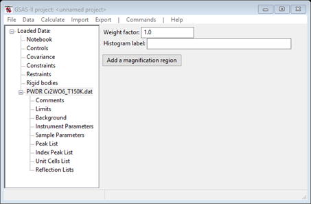
and the plot window will show the powder pattern

We will leave the limits alone for this purpose.

Step 2. Read in the chemical structure for Cr₂WO₆

1. Use the Import/Phase/from CIF file menu item to read the phase information for Cr₂WO₆ into the current GSAS-II project. This read option is set to read Crystallographic Information Files (CIF). Other submenu items will read phase information in other formats. Because you used the Help/Download tutorial menu entry to open this page and downloaded the exercise files (recommended), then the Magnetic-II/data/... entry will bring you to the location where the files have been downloaded. (It is also possible to download them manually from https://subversion.xray.aps.anl.gov/pyGSAS/Tutorials/Magnetic-II/data/. In this case you will need to navigate to the download location manually.)

2. Select the Cr2WO6.cif data file in the first dialog and press Open. There will be a Dialog box asking Is this the file you want? Press Yes button to proceed. You will get the opportunity to change the phase name next (I changed it to Cr2WO6!); press OK to continue.

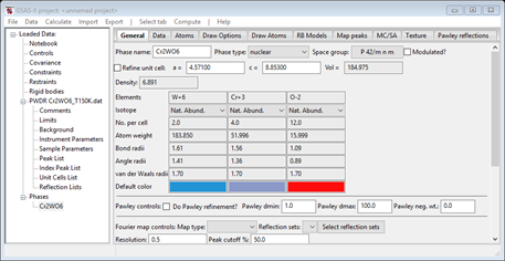
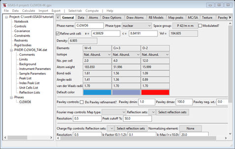
3. Next is the histogram selection window; this connects the phase to the data so it can be used in subsequent calculations. Select the histogram (or press Set All) and press OK. The General tab for the phase is shown next

Step 3. Structure refinement

We are now ready for initial refinement of scale and background. Do Calculate/Refine from the main menu; a File Selection dialog will appear wanting a file name for your project. I used Cr2WO6 150K; the refinement proceeded quickly. The fit is quite poor (wR ~46%), mostly from bad peak positions. This is a combination of lattice parameters being smaller at 150K vs room temperature and sample placement on the goniometer. Find the Sample Parameters entry in the tree change the goniometer radius to 1000 and set the refinement boxes for Sample X & Ydispl. Then go to the Cr2WO6 phase and set the lattice parameter refinement. Do Calculate/Refine; the residual will be much improved (wR=12.9%). Interestingly, the sample position is displaced by ~ -5.9mm along the X-direction & ~ -1.8mm in the Y-direction. Finally, go to the Atoms tab and set refinement flags X & U for all atoms. Do Calculate/Refine; the residual will be a bit better (wR = 11.69%). We are done with this step; Save the project & close GSAS-II; we will use this phase information for the magnetic structure study.

The magnetic structure of Cr₂WO₆

Step 1. Read in the data file

1. Use the Import/Powder Data/from TOPAS xye or Fit2D chi file menu item to read the data file into the current GSAS-II project. This read option is set to read the powder data format used by Topas, etc. Because you used the Help/Download tutorial menu entry to open this page and downloaded the exercise files (recommended), then the Magnetic-II/data/... entry will bring you to the location where the files have been downloaded. (It is also possible to download them manually from https://subversion.xray.aps.anl.gov/pyGSAS/Tutorials/Magnetic-II/data/. In this case you will need to navigate to the download location manually.)
For this tutorial you will not see the data file in the file browser, because the extensions on data files are not the expected ones, you will need to change the file type to All files (*.*) to find the desired file.

2. Select the Cr2WO6_T4K.dat data file in the first dialog and press Open. There will be a Dialog box asking Is this the file you want? Press Yes button to proceed.

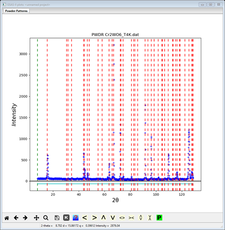
3. Since this data file does not define an instrument parameter file, a file dialog will appear for you to select the correct instrument parameter file. Select Cr2WO6_T4K_dat.prm; you may have to change the file type in the file selection Dialog box to GSAS iparm file to see it. At this point the GSAS-II data tree window will have several entries

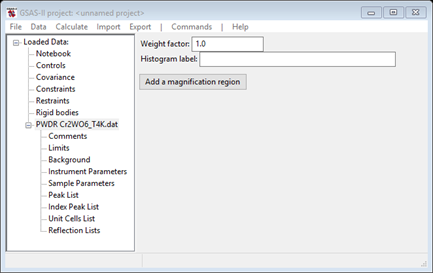
and the plot window will show the powder pattern

We will use the default limits.

Step 2. Read in the chemical structure for Cr₂WO₆

1. Use the Import/Phase/from GSAS-II gpx file menu item to read the phase information for Cr₂WO₆ into the current GSAS-II project. The file you want is the one from the 1^st part of this tutorial and should be in your current directory. This read option is set to read from other GSAS-II project files. Other submenu items can read phase information in other formats.

2. Select the Cr2WO6 150K.gpx data file in the first dialog and press Open. There will be a Dialog box asking Is this the file you want? Press Yes button to proceed. You will get the opportunity to change the phase name next; press OK to continue.

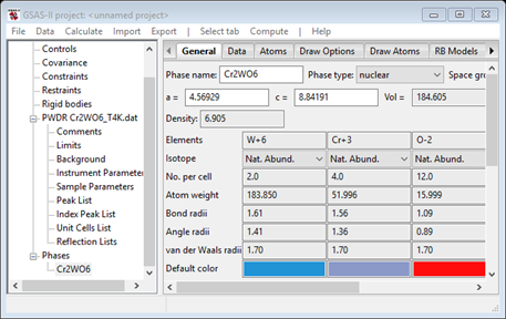
Next is the histogram selection window; this connects the phase to the data so it can be used in subsequent calculations. Select the histogram (or press Set All) and press OK. The General tab for the phase is shown next

Step 3. Check powder pattern indexing

Here the objective is to determine how the reflection positions generated from the chemical (“nuclear”) crystal structure lattice match up with the peaks observed for this antiferromagnet.

1. Select Unit Cells List from the tree entries under the histogram (begins with PWDR); the Indexing controls will be shown

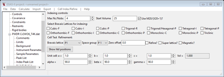
This can be use lattice parameters & space groups to generate expected reflection positions to check against the peaks in the powder pattern.

2. One could then enter Bravais lattice, choose space group & enter lattice parameters by hand, but the easy way is to use the chemical lattice directly. Do Cell Index/Refine/Load Cell from the menu; a Phase selection box will appear with only one choice (Cr2WO6). This was taken from the Phases present in this project; there could be more than one depending on what you loaded/created earlier. The Import menu item allows you to get lattice information from any one of the other phase containing files known to GSAS-II. Press OK and the Indexing controls will be change

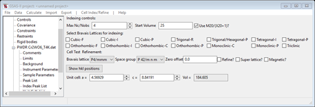
showing the lattice constants for Cr₂WO₆ you had obtained from the gpx file and the powder pattern will change showing the lines for P 4₂/m n m and the LaMnO₃ lattice parameters. Change the space group to P 4/m m m; the plot will change showing the new lines.

Notice that every peak (apart from some junk!) is indexed, especially the intense lowest angle peak. Put the cursor on it to identify it (001) as that will be useful in selecting possible magnetic structures. In this case ones with only mz allowed by symmetry are not the correct ones. No doubling of the unit cell along any axes is needed, this makes the magnetic propagation vector, kx ky kz = 0,0,0; this will be needed in the next step.

3. Reset the space group back to P 42/m n m (VERY IMPORTANT!) you may do a Load Cell again if you wish).

Step 4. Run k-SUBGROUPSMAG

In this next step, you will be accessing the Bilbao crystallographic server so you must be connected to the internet. In the Cell Index/Refine menu select Run k-SUBGROUPSMAG; a small popup dialog will appear

These are the controls for running the Bilbao routine. The space group is taken from the Space Group entry on the Unit Cells window. Since we did not discover any cell doubling, leave the kx ky kz entries as they are. Do select Cr+3 from the test for mag. atoms pulldown as that will restrict the models to those with a nonzero magnetic moment on the Cr atoms. We will discuss the other options in another tutorial. Press Ok. A popup dialog will appear reminding you how to cite the Bilbao routine in any paper you write using this facility.

Press Ok, the nag note will also appear on the console and after a pause, the console will show “request OK” indicating that the Bilbao site has responded with some results. GSAS-II will next display a File Dialog asking for a project name to save this project; change the directory to a useful place for your work on this tutorial and give the project a name; I used Cr2WO6 4K.

The GSAS-II data window will display the results from k-SUBGROUPSMAG. (If k-SUBGROUPSMAG failed because you lack internet access, this file is located in the same location as the powder data and cif files used above were found. Do File/Open Project from the main menu to access it as “Cr2WO6 4K.gpx”).

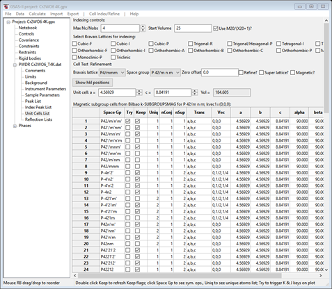
The table shows all the magnetic space groups that are possible starting with P 4₂/m n m and zero propagation vector; this is noted in the table heading. Notice that it goes all the way to a triclinic P1 magnetic space group; you probably will never need to go that far to find a suitable magnetic space group. The ones marked ‘Keep’ have a possibly magnetic Cr atom based on the magnetic site symmetries of the transformed atom positions (there may be more than one – see the Uniq column for how many there are). Each entry also shows the transformation matrix in symbolic form and the necessary origin shift so that the new structure is properly positioned to satisfy the new space group. There are ~90 entries in this table; one of them is the correct one so we have some searching to do.

Step 5. Checking indexing

The process here is simple (if a bit tedious); simply select Try for any row marked Keep. If the calculated pattern doesn’t index the peaks (especially the 1^st one), unKeep it and try the next one. Go at least as far as the 64^th row which covers the tetragonal and orthorhombic space groups. Alternatively, one could change the filters on the space groups to be Keeped by only choosing those with just one magnetic Cr (see the Uniq column for these). Double click the Keep column heading; a small popup dialog will appear

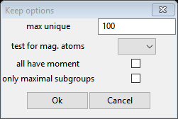
Enter 1 for max unique and select Cr+3 from the test for mag atoms item; then press Ok. The Unit Cell List will be redrawn

Now do the Try of each one marked Keep; there are fewer than before since only those with 1 Uniq are marked Keep.

There are no tetragonal ones and only 4 orthorhombic ones that index the pattern. Most likely, the correct one will have only one Cr atom position with m_x and/or m_y moments allowed; no solutions with just m_z are permitted because the 001 reflection is strong. To find the correct one we have to try to create magnetic phases for each examining the Cr atom moments with this criteria.

Step 6. Select 1^st magnetic structure

Select the Cr2WO6 phase from the GSAS-II data tree (under Phases). The General tab is shown for this nuclear phase.

Do Compute/Select magnetic/subgroup phase; that will make a small popup dialog

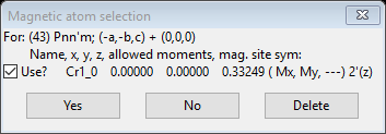
This shows all magnetic phases that were marked Keep in the Unit Cells List; for each you see the transformation and vector (occasionally two results will have the same space group but are different translations). Select the 1^st one and press OK; a new popup dialog will appear.

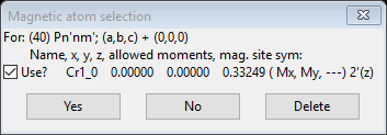
This one, #40 P n’nm’, has Mx & My allowed moments on a single Cr atom. Press Yes. The project will be saved first, then a file dialog box will appear offering a project name for this magnetic structure. It is named with the number from the space group list; press Save. The new project will be opened to the General tab for Pn’nm’ magnetic phase just created.

Now select the Atoms tab for the magnetic phase

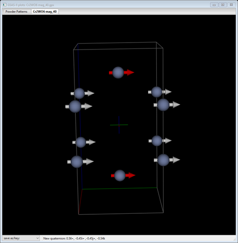
You’ll see that both Mx and My are allowed; there is no easy clue from the diffraction data where the moment lies so we’ll just have to try something. A useful thing to do is to try individually Mx=1 & My=0 and vice versa each time drawing the unit cell contents. Select the Atoms tab for the magnetic structure and change Mx=1, My=0. Then select the Draw Atoms tab

Select the one atom and do Edit Figure/Fill unit cell; the table will list 10 atom positions and the drawing will show

This is an antiferromagnetic structure. Now select the Atoms tab and change Mx=0, My=1; the drawing will update the moments

which is now a ferromagnetic structure. Clearly, this is not correct since we know the material is an antiferromagnet. Therefore, in Pn’nm’ My=0 and Mx > 0. So we should try refining Mx with My fixed. Change Mx=1 and My=0 and select the M refine flag. Then go to the Constraints entry

Do Edit Constr./Add hold for 1::Amy:0. Now do Calculate/Refine. The residual is quite poor wR~39%) and Mx did not change much. Even after including refinement of the rather large sample displacements (recall the 150K refinement) wR ~ 28%. Perhaps this isn’t the correct structure, so let’s look for another. Save the project (it still might be useful).

Step 7. Select 2nd magnetic structure

To continue the selection process, we need to use the saved project used for the first selection because it contains the table of possible magnetic space groups generated by k-SUBGROUPSMAG. Do Open project from the main menu and select Cr2WO6.gpx; you’ll see a reminder to save the old project (we just did this) and select the Cr2WO6 phase (should be the only one); the General tab will be shown

Do Compute/Select magnetic phase from the menu; the popup should look like

We have already tried #40 (Pn’nm’), so let’s try (43) Pnn’m next. Select it and press OK; a popup will appear

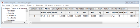
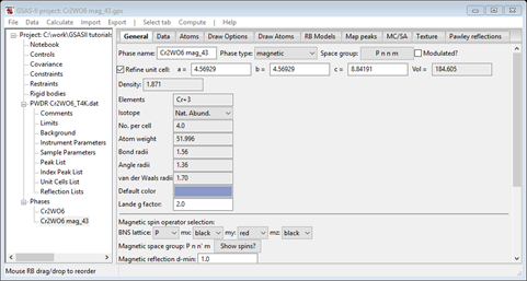
This is similar to #40; one magnetic Cr atom with allowed Mx & My moment components. Press Yes. The project will be saved and a new project Cr2WO6 mag_43.gpx will be created. The General tab for this new phase will be shown

Select the Atoms tab

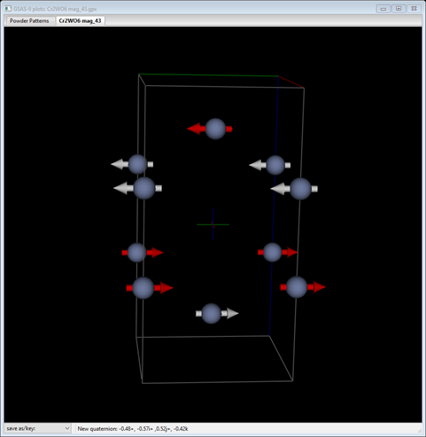
Again Mx & My are allowed moments but we don’t know what their values are. We can try drawing each; set Mx=1 & My=0. Select the Draw Atoms tab, select the Cr atom and do Edit Atoms/Fill unit cell; the drawing will show

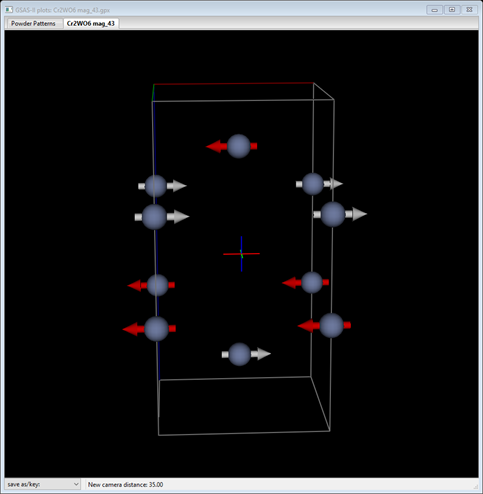
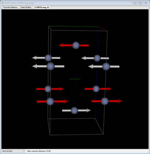
which is an antiferromagnetic structure. Now try Mx=0 and My=1; the structure will show

which is yet another antiferromagnetic structure. We can try each one or just set Mx=1 and My=1 and refine both to see where it goes. Set Mx=1, My=1 and clear any refinement flags in both phases (see General & Atoms for both phases). Do Calculate/Refine from the main menu; wR is ~39%. Next, set the M refinement flag for the magnetic Cr atom and repeat Calculate/Refine; wR drops to ~37%. Most importantly, Mx is close to zero and My ~2.3. Add the sample displacement parameters (set radius to 1000) and refine again. wR drops to ~ 23% which is much better than a similar refinement for #40 (~ 28%).

Moreover, the 001 magnetic reflection has considerable calculated intensity; the overall fit is pretty good (except for perhaps lattice parameters). Next we will complete the refinement using this solution.

Step 8. Complete refinement of structure #43 (Pnn’m) for Cr₂WO₆

From what we noticed about the initial refinement for this solution, Mx=0 and needs to be held there. So select the Atoms tab for the magnetic phase

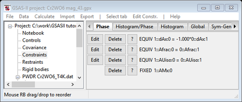
Set Mx=0. Next, select the General tab for each phase and check the Refine unit cell box for each. Next, we have to set the hold on Mx; select Constraints

Notice the two constraints which ties the two normally inequivalent orthorhombic metric tensor elements to a single tetragonal one. Now finally add the hold on Mx; Do Edit Constr./Add hold; select 1::AMx:0. The constraints should look like

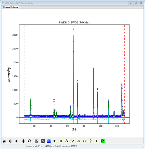
Now do Calculate/Refine; the residual immediately drops to 12.2%. Finally, add refinement of atom positions and Uisos to both phases and repeat Calculate/Refine. My residual is 11.75% and the plot shows a nice fit for this magnetic structure

The remaining misfits are from some contaminating phase(s) because they are not indexed by either the chemical or magnetic phases. A bit more improvement can be made by using 6 background terms and including the U, V, W and SH/L instrument parameter coefficients. My wR was ~11%. The magnetic structure is

The Cr magnetic moment (m_y) = 2.35(2) shown in Cr2WO6 mag_43.lst. Notice that the chemical space group is tetragonal; although the effect is very small, the magnetic ordering will reduce the chemical cell symmetry to match the magnetic symmetry. The analysis presented here gives the proper subgroup needed for this description, Pnnm, along with the transformation (a,b,c)+0,0,0. This concludes this tutorial; you may wish to save the project.