Le Bail Intensity Extraction in GSAS-II - Sucrose

· Exercise files are found here. The data files are also used in the 3rd section of the Fit Peaks/Autoindexing tutorial.

Background

In a Rietveld fit, a number of different items are fit, potentially at the same time. These include the lattice parameters, atomic positions and displacement (aka “temperature”, U_iso and U_ij) parameters for one or more phases, as well as peak shapes parameters either for broadening from either the sample or the instrument (avoid doing both together), background fitting terms and one or two correction terms needed to describe peak shifts due to apparent sample placement. In addition, there could be other terms needed to describe additional experimental conditions such as for absorption, preferred orientation or extinction. These parameters can be divided into four categories: experimental (peak shapes, peak shifts and background), lattice parameters, structural parameters (atom positions and U values) and intensity correction terms (absorption, preferred orientation and extinction).

In Rietveld, the reflection intensities are generated from the structural and intensity correction parameters, but there are two approaches to full-pattern fitting that treat reflection intensities as arbitrary: (1) Pawley fitting, developed by Stuart Pawley [Pawley, G. S. (1981). "Unit-Cell Refinement from Powder Diffraction Scans." Journal of Applied Crystallography 14: 357-361.], where peak intensities are treated as least-squares variables. (2) Le Bail fitting, from Armel Le Bail [Le Bail, A. (2005). "Whole powder pattern decomposition methods and applications: A retrospection." Powder Diffraction 20(4): 316-326.] The Le Bail approach, demonstrated by this tutorial, takes advantage of the fact that Hugo Rietveld developed a rather ingenious approach to estimating reflection intensities: the idea behind this is that for every point in a pattern where one or more reflections contribute, one can estimate the relative contribution from each reflection from the structure factor magnitude, F²_calc, from the approximate crystal structure model, adjusted for reflection multiplicity (m), preferred orientation and various other geometric corrections. Simply apportioning the observed powder pattern intensities point by point to each reflection provides an estimate for the observed structure factors, F²_obs. The quality of this estimate improves as the crystal structure model approaches reality. Le Bail’s method cleverly appropriates Rietveld’s intensity extraction, but assuming the crystal structure model is unknown, sets all F²_calc values to an initial value (e.g. 1.0). After the intensity extraction is performed, a set of F²_obs values is obtained. These initially treat every F²_obs/m ratio as equivalent and will not be very accurate, but they are much better reflection estimates than the initial F²_calc values (all unity). The F²_calc values are set to the extracted F²_obs and the Le Bail fit can be repeated, giving even better intensity estimates. This process is equivalent to a steepest descents minimization and it will converge to a self-consistent set of intensities that will give best possible agreement to the observed pattern. Note that the apportionment of intensity for reflections that are very closely overlapped will tend to make their F²_calc values approximately equal. (Note that the Pawley approach will tend make m*F²_obs values equal for complete reflection overlap; neither is likely to be accurate.)

Note that when either Pawley or Le Bail intensity extraction are used, the structural and intensity correction parameters no longer affect the intensity computations. Such parameters should not be included in the fit as they will produce singularities in the refinement. If included inadvertently, GSAS-II will usually remove them from the fit along with providing annoying warning messages, but it is possible that this parameter removal process could fail and the refinement may not run properly.

After the LeBail option has been invoked, the Calculate/Refine menu command will execute a preliminary LeBail only “zero cycles” refinement in which only F²_obs is adjusted via the LeBail method. It is cycled 10 times or until a minimum is reached. After that completes, the Rietveld/LeBail refinement proceeds allowing least-squares minimization of non-intensity dependent parameters toward a more global fit to the data. Successive runs allowing other parameters to be varied can then be used to progressively improve the fit and produce a best estimate of the F²_obs.

There are many reasons to use Le Bail fitting. The technique was developed to obtain a set of reflection intensities for structure solution. It can also be used to treat an impurity, where lattice parameters are known but the structural details are not or for fitting lattice parameters where likewise the structure is not known. Le Bail fitting is also useful prior to a structural fit. It can allow determination of reasonable starting values for the background, peak shapes and unit cell parameters so they can be fixed until the late stages of the refinement, although the freedom in peak intensities may bias some parameters (e.g. background and profile coefficients) if there is a large number of overlapping reflections. Another use is to see when artifacts in the background or peak shapes limit how well the pattern can be fit. A Le Bail or Pawley fit provides an estimate for the best possible R_wp and reduced χ² values that can be expected for a dataset. For complex patterns, where it is difficult to discern where allowed reflections are present, comparison of Le Bail or Pawley fits can provide insight on extinction conditions. A lower symmetry space group with fewer extinctions should provide a better fit to warrant its consideration.

Prerequisite

In this exercise you we will use Le Bail fitting to extract approximate reflection intensities. This is similar to what is done in the beginning of the “Charge Flipping in GSAS-II - sucrose” tutorial, which instead uses Pawley fitting. It follows logically from the third example in the “Fit Peaks/Autoindexing in GSAS-II” tutorial, from where the sucrose unit cell was determined. Alternately, a project (start.gpx) file is provided in the exercise files to start without the previous tutorial.

Step 1: Setup for fit

From the final project file, after completing the indexing and creating the phase, make the the following changes:

· Controls: Set the “Max cycles” value to 5

· Limits: Raise the upper data limit from 8 to 24 degrees

· Background: Add a background peak at 5.5 deg with sigma=10,000, set the flag to refine the peak intensity. This is to accommodate a broad peak in the background from the Kapton capillary used to hold the sucrose sample.

· Instrument parameters: Use the Operations/Reset profile menu command to return to the beamline-supplied terms; turn off refinement of all terms

· Sample parameters: turn off refinement of the histogram scale factor and make sure the goniometer radius is 1000 mm.

· Phase Sucrose/Data tab: Use Edit phase/Add powder histograms to link this phase to the powder dataset; set the refine flag on for the size term and the microstrain term.

· Phase Sucrose/General tab: Set the Refine unit cell flag.

These changes have been applied to a GSAS-II project file from the conclusion of the 3rd Example within “Fit Peaks/Autoindexing in GSAS-II” tutorial and is provided as for this tutorial as file start.gpx.

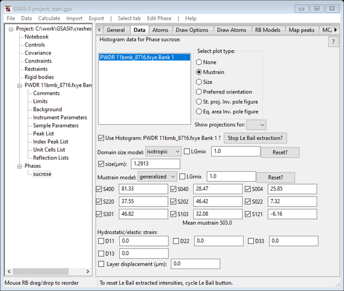
Step 2: Select Le Bail fitting

On the phase Data tab, press the Start Le Bail extraction? button to put the refinement into Le Bail mode.

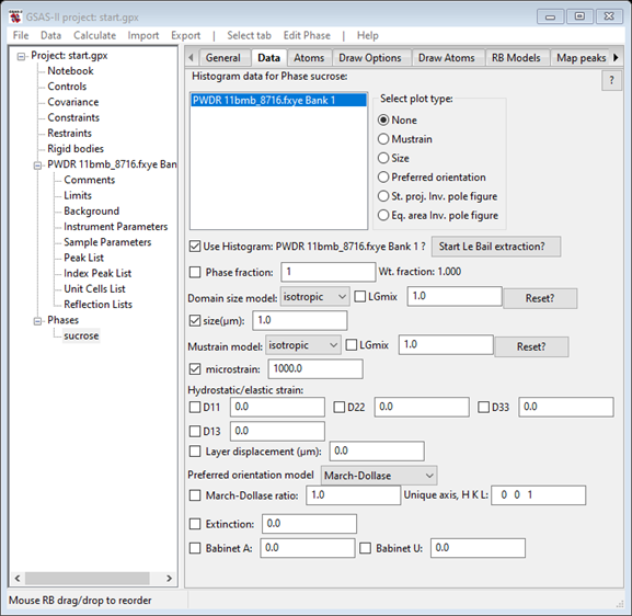
The window will be redrawn with all intensity dependent variables removed from view

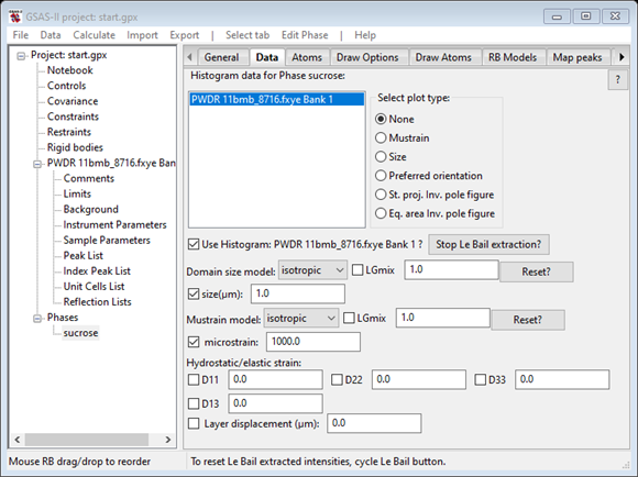
and the LeBail button has changed to “Stop LeBail extraction?”.

Step 3: Do the initial Le Bail fit

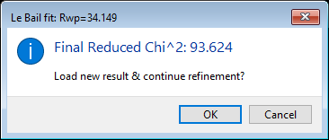
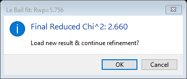
Do the Calculate/Refine menu command. A popup message will appear informing you that it will do the initial zero cycle LeBail fit of the intensities.

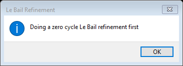
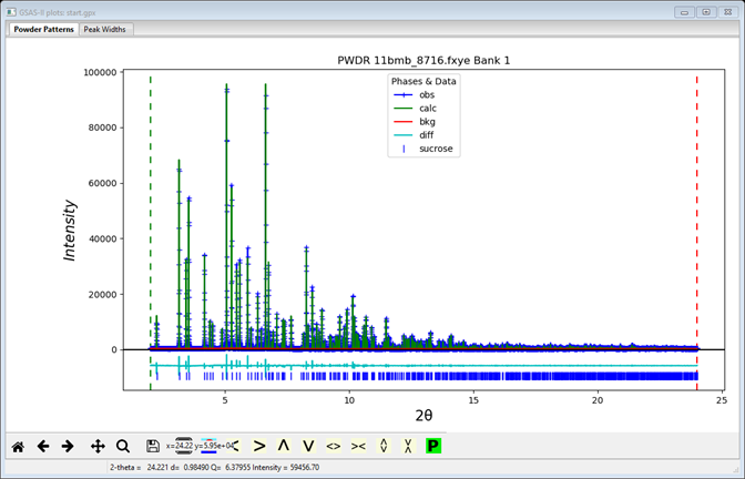
press Ok. The refinement will proceed and yield Rwp ~34%. The popup has an Ok and Cancel buttons. The plot has been updated with this fit.

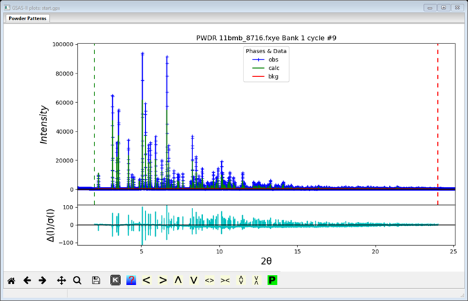
You should have a look to be sure that the peaks are in the right places and that some calculated intensity is present under them. Otherwise you should press Cancel & adjust things as appropriate (e.g. lattice parameters).

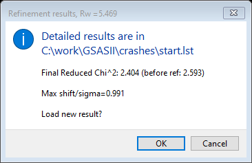
Press Ok to save this & proceed to the 1^st full Rietveld/LeBail refinement. The next refinement will include those parameters you selected for a full Rietveld/LeBail refinement. The initial residual should be where the initial LeBail fit finished. This will run through five cycles of Rietveld/Le Bail fitting and the residual will drop to Rwp ~12.6%

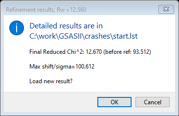
and the fit will be much improved

Press OK to accept these results.

Step 4: Add more parameters

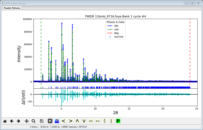
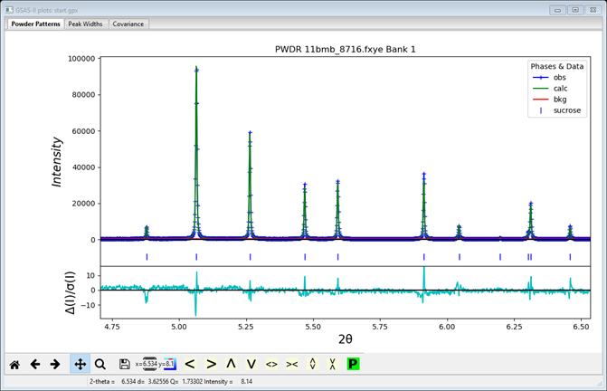
Clearly, further improvement in the fit is desirable. Closely examining the fit shows issues with background, profile shape and peak positions.

Plotting the (obs-cal)/sigma curve (press the w key) and enlarging it (use the crossed-arrows button and drag the right mouse button upwards inside the lower box), as shown above, shows that further background improvement might be expected with more background terms.

· Change to use 6 chebyschev-1 parameters.

· Also refine sig and pos for the single background peak.

The peak positions are probably offset from a sample position error (it is almost always present)

· Select Sample X displ in Sample Parameters

The peak shape shows perhaps (in this case) inadequately determined instrumental U, V & W parameters

· In Instrument Parameters select U, V & W for refinement.

Do Calculate/Refine; there will be a high residual for the initial steps but will quickly settle down to Rwp ~ 6.0%

Pretty clearly, this sucrose sample gave an instrumental profile that was better than what the provided instrument parameter file indicated

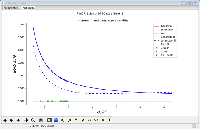
The solid line is from the default set of instrument parameters, the crosses are from the single peak fits done in the peak fitting tutorial and the dashed curve is from the results of this fit.

Step 5: Explore peak shape terms

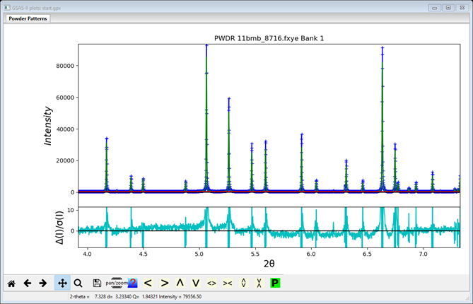
At this point the fit is still poorer than what would be expected based on counting statistics (which would yield a reduced χ² value close to 1.) Looking closely at the data and computed pattern, as shown below for example, leads one to believe that the profile is still not being well-fit.

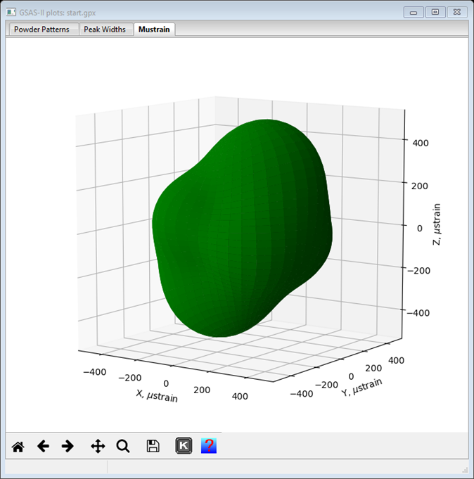
A Le Bail fit provides a good way to explore different peak shape broadening options. Moreover, if the intended use of the extracted structure factors is structure solution, then one wants the best LeBail fit possible. Investigation of a number of models for anisotropic peak broadening finds that the R_wp can be reduced to 5.23%, through use of the Popa/Stephens model for microstrain (refining 9 terms in the generalized mustrain model), with a plausible microstrain directional plot, as below. A fit that uses fewer terms that is almost as good uses uniaxial crystallite domain size broadening along the 010 axis and uniaxial microstrain broadening along the 010 axis, my residual was R_wp = 5.38%. This adds 2 only parameters. We will continue with the isotropic size and generalized mustrain models; my final R_wp after several sets of LeBail/Rietveld refinement was R_wp = 5.197%.

The important result here is that this sample exhibit non-ideal broadening artifacts. This could be due to milling of the sucrose during manufacture creating defects that cannot be well-fit with a conventional peak shape. From this fit, it is now clear that best possible fit to be expected from any structural model will have a R_wp on the order of 5% and a reduced χ² value on the order of 1.5, since no crystal structure model could give a better intensity fit than a Le Bail or Pawley fit.

Step 6. Resetting the LeBail extracted intensities

A perhaps further improvement in the extracted structure factors with the aim of using then in structure solution can be obtained by reinitializing the LeBail extraction using the now better parameter set. Go to the Data tab.

Notice the message on the righthand status line; to reset the LeBail intensities, “cycle” the Le Bail button. Press Stop Le Bail extraction (NB: this will set the refinement into normal Rietveld mode – impossible because the model contains no atoms!). The window will be redrawn to include the intensity dependent parameters. Now press it again (Start Le bail extraction?). The window will be redrawn again. The next refinement will start with new initial structure factor values (=1.0) and will do the preliminary “zero cycle” Le Bail refinement. You may leave the refinement parameters alone. The refinement will start out high (Rwp~67%) but will quickly drop to ~5.7% because all the other parameters are near their optimal values.

Press OK to continue with the Rietveld/LeBail part of the refinement; a popup will show the status of this part.

Press OK. Set the number of cycles to 20 and repeat Calculate/Refine until the fit has converged (it may take several repeats as this part of a Le Bail refinement does converge slowly). I got Rwp = 5.26% when I quit recycling the refinement. You can now use these extracted intensities to see if they can be used for a charge flipping structure solution (I did get it to work once – otherwise many failures).