Determining Profile Parameters from Fundamental Parameters

The goal of this exercise is to determine approximate instrument profile parameters by calculating peak profiles based on a fundamental parameters approach (FPA) description of a diffractometer. The peaks are then fit using the profile model terms within GSAS-II. Note that with fundamental parameters, it is possible to generate highly irregular peaks that GSAS-II will not be able to fit well. It is best to use instrument configurations that produce well-formed peaks, which can be modeled by a Voigt functions with the addition of asymmetry from angular divergence.

The FPA peak shapes are computed with the NIST FPA Python code (http://dx.doi.org/10.6028/jres.120.014.c), which should be cited using "Mendenhall, Marcus H.; Mullen, Katharine; & Cline, James P.; (2015). An Implementation of the Fundamental Parameters Approach for Analysis of X-ray Powder Diffraction Line Profiles.120 223-251. 10.6028/jres.120.014," if this capability is used within GSAS-II. This code is used to generate a pattern with isolated peaks. The profile of these peaks is fit using profile parameters U, V, W, X, Y and SH/L.

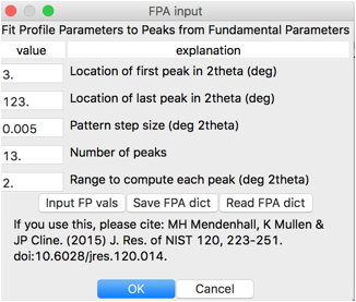
1. Open the FPA module

To invoke this capability, the "Import/Powder Data/Fit instr. profile from fundamental parms…" menu command is used. This opens a dialog, as below

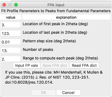
This describes how a pattern will be generated. The computation should be done over the angular range at least as large as the data range for analysis of samples. Since we will fit several profile terms, at least double that number of peaks should be computed. The default of 13 peaks, to space them 10 degrees apart, works well here and would not need to be increased if a larger data range were used. Lowering this number might be needed to keep peaks from overlapping, if very broad peaks and a small data range are used. The pattern step size should allow at least 10 points above the half-intensity point in each peak, which would need to be made smaller with narrow peaks. As will be shown, this is checked, so leaving this as the default value is fine. Computing each peak over a 2-degree range is likely way more than what is needed in this example, but also does not slow the computation noticeably. This might need to be changed with very broad or very narrow peaks. For this example, we will not change any parameters.

2. Input FPA parameters

The FP parameters can be input in one of two ways. They can be read from a file, which can be hand-edited to access the full range of capabilities in the NIST FPA Python code (discussed further in "7. Supplying NIST FPA input manually" below) or can be input from another dialog window. Press the "Input FP vals" button, which opens the window shown below:

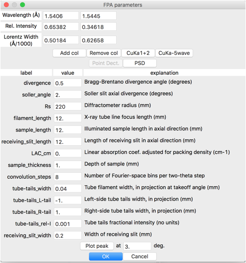
The top section of the dialog window specifies the details of the radiation source, where any number of components can be given. Two common default settings with Cu Kα radiation modeled as a 2-line or 5-line spectrum. The input can also be switched from Point-detector mode (as is shown above) to position-sensitive-detector mode, by pressing the PSD button. Note that parameters are named similar to their use in the Topas program with the same units.

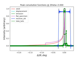
3. Plot the peak shape and convolution contributions (optional)

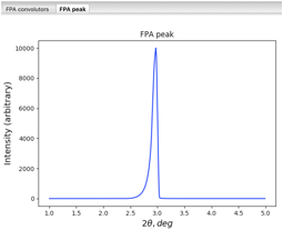
The "Plot peak" button at the bottom of the window can be used to visualize the resulting peak shape at any position in 2-theta, as well as all the contributions to the peak shape, like this:

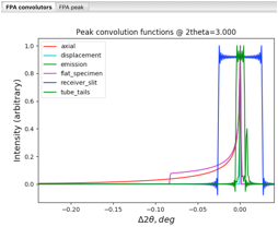
Note that distinguishing the components in the peak convolution functions plot can be difficult. Clicking on an entry in the legend changes the display of that component, as shown below where "emission" in the legend was clicked:

4. Accept the FPA values, correct the step size

For this example, we will not change any of the default FPA parameters. Press OK to accept the displayed values and to close the dialog window. The pattern step size is then checked, producing the following warning:

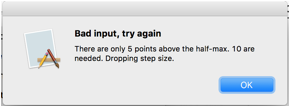
Note that the Pattern step size is changed, as below.

Also note that after values have been entered, the "Save FPA dict" button is now available.

5. Perform the computation

Press OK to start the computation. A "please wait" message is displayed

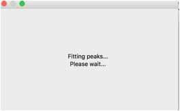
as the fitting may take a few minutes (output can be seen in the console window as the fit progresses). When the fit is complete, you will be provided with a window to save the instrument parameters to an .instparm file. After the parameters have been saved, the fit will be plotted (here I have switched to the main PWDR tree entry and dragged the difference curve down so that it can be seen better.)

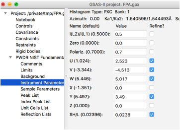
Clicking on the Instrument Parameters tree entry causes the powder profile terms to be plotted:

6. Improve the profile parameters.

Note that due to correlation between the peak asymmetry parameter (SH/L) and the Lorentzian broadening terms, the Gamma (Lorentz width) terms refine to negative values for the first few low angle peaks. This can be addressed by setting X to 0.0 and refining U, V, W, Y and SH/L but not X in the "Instrument Parameters" tree item. Then return to the "Peak List" tree item to use the Peak Fitting/Peakfit menu command. Finally, return to "Instrument Parameters" and use Operations/Save Profile to write the improved values to an .instparm file.

7. Supplying NIST FPA input manually.

Once FPA values have been entered, the "Save FPA dict" button can be pressed. The contents of this file, slightly reformatted for more easy reading, is shown below. Note that the dict keys and values use the naming and SI units from convolutors the NIST FPA program. By editing this file, it is possible to use all of the convolution features within the NIST program, beyond the values that can be edited from the GUI.