A video version of the first two parts of this tutorial is available at https://anl.box.com/v/FindProfParamCW
Exercise files are found here
The goal of this exercise is to determine approximate instrument profile parameters for a lab instrument by a simple peak fit to a standard sample. Then in the step labeled Save Instrument Parameters a new instrument parameter file is created, allowing these parameters to be used as the starting point for refinements with other datasets. Ideally, one should use a material or mixture of materials that has peaks over the entire range where you collect data and use material(s) that have negligible sample broadening (from crystallite size or microstrain. The NIST LaB\(_6\) standards (SRM 660, 660a and 660b,…) are good choices for this, as they have very little sample broadening and a relatively small number of peaks but over a wide angular range, although it would be good to have a pattern with peaks starting a somewhat lower in \(2\theta\).
While older refinement codes used a single set of profile terms, which treated both sample and instrumental broadening, GSAS-II offers a much-improved mode of use, where these terms are separated into different sections of the parameter arrays. (The sample terms are available for each phase and for each histogram and are found in the Data tab for each phase.) GSAS-II does allow for the older mode where both effects are treated by a single set of terms, but this is creates for much difficult refinements. With the new mode, the instrumental terms can be fit once for an instrumental configuration and then they do not need to be refined with other samples, making the fit much simpler to perform and allowing the sample’s crystallite size and microstrain contributions to be quantified. This tutorial shows how these instrumental terms may be determined and saved for future use.
GSAS-II uses a so-called pseudo-Voigt peak shape, where Gaussian and Lorentzian (the term Cauchy is also sometimes used for Lorentzian) contributions to the peak shapes are added. In reality, the Gaussian and Lorentzian contributions are convoluted which yields a Voigt peak shape, but the pseudo-Voigt function is a very good approximation of the Voigt and is much simpler to compute. Also, for almost all diffraction instruments and samples, instrumental broadening is Gaussian while sample broadening is Lorentzian. For the Instrumental Parameters, the U, V & W terms provide Gaussian broadening and the X & Y terms provide Lorentzian broadening. (Hence X & Y are expected to be zero when the Instrumental Parameters are not accounting for sample effects.) When performing individual peak fits, the Gaussian broadening is determined by the \(\sigma^2\) term and the Lorentzian broadening is determined by the \(\Gamma\) term, as described in the GSAS-II help pages.
Note that it is highly recommended to collect reference data to a much higher \(2\theta\) angles than the data used in the example here. What is done in this example would be sufficient only if one will never collect and use data above 70\(^\circ\) degrees (this is unlikely!).
To get started, create a new project in GSAS-II, either by starting the program fresh or using File/New Project.
Use Import/Powder Data/from Bruker RAW file to read
file LaB6_Jan2018.raw from the Tutorials CWInstDemo/data
directory (download from https://advancedphotonsource.github.io/GSAS-II-tutorials/CWInstDemo/data/).
After selecting this file, answer Yes to the question “Is this the file
you want?”
The next dialog to appear is titled,
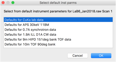
Choose inst. Param file for LaB6_Jan2018.raw Scan 1 (or Cancel for default).
Since we do not have a set of instrument parameters to read, we must
start from one of the default set of parameters that GSAS-II provides.
Press Cancel for this dialog window. This raises the
default Inst Parms dialog:
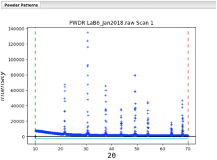
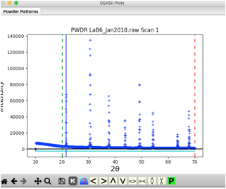
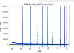
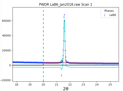
Here, choose the first option for CuKa lab data (which is for a standard instrument with K\(\alpha_1\) and K\(\alpha_2\) radiation). Then press OK. A plot of the data will appear as to the right:
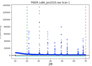
Note that the data begins at 10\(^\circ\), but the first peak is above 21\(^\circ\). So we can simplify the background fitting by changing the data limits. Click on the Limits data tree item, and either change the Tmin value from 10 to 20, or in the plot “drag” the green line to the right to approximately 20\(^\circ\).
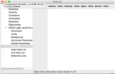
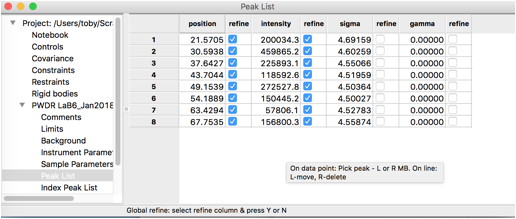
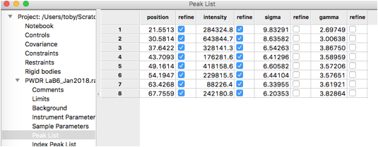
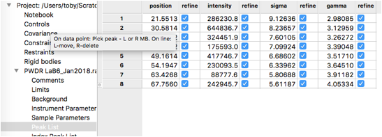
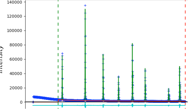
To define peaks, click on the “Peak List” data tree item. Note that as below, the peak list is initially empty.
Move the mouse to any of the data points close to the top of the first peak and click the left mouse button. A blue vertical line will be drawn through the peak, as to the right, and the position will be added to the peak table.
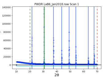
Repeat this for all 8 peaks in the pattern. Note that if a peak is entered in the wrong place it can be moved by “dragging” it with the mouse, or use a right-click to delete it. Be careful to make sure two peaks are not entered in the same place by accident.
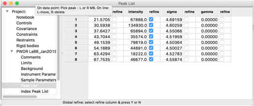
The peak table appears as to the right.
By default, the peak intensities are flagged as to be varied, but not
any of the other parameters. We will eventually fit peak positions and
widths in addition to intensities, but It is wise to make sure each set
of parameters has a chance to converge before adding more, so we start
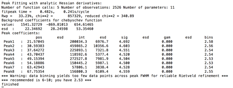
with only the intensities. Use the Peak Fitting/Peakfit
menu item to perform a peak refinement. You will be asked for a name to
save the project. (Enter a name such as peakfit.gpx and
press Save). The peaks are then fit, here optimizing only the intensity
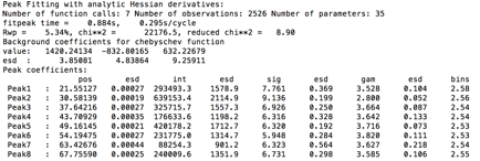
values. The console window shows the details of the refinement:
The warning shown at the end is because the default peak parameters describe a peak shape that is significantly sharper than what is actually present for these data; the step size for these data is actually fine. This warning will later go away, but if it did not, this would indicate that it would be better to recollect the data with a step size decreased.
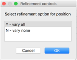
In the peak list window, double click in the refine heading for the peak position flags, this will bring up a dialog that allows all peak positions to be varied.
Select “vary all” and press OK. Now all peak positions and areas will be refined. Use the Peak Fitting/Peakfit menu command to start peak refinement. Note that control-P (on Mac command-P) is a shortcut for the Peak Fitting/Peakfit menu item.
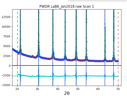
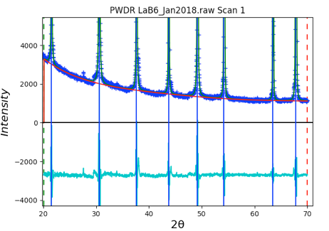
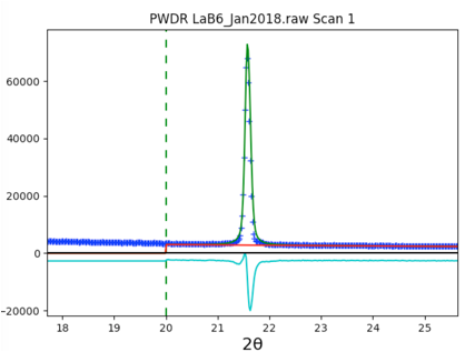
The fit improves significantly, as shown to the right, but a good fit requires also fitting peak widths.
We could at this point proceed to fit the instrumental profile terms, so this next step can be skipped, but for the purposes of showing how individual peak fitting is done, we will try this first. It does have the advantage as it will show if any peaks have anomalous widths.
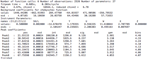
Double-Click on the refine headings for the sigma2 (Gaussian width) and gamma (Lorentzian width) parameters so that all parameters can be refined. Use the Peak Fitting/Peakfit menu item to again start peak refinement. The results in the console window are shown to the right.
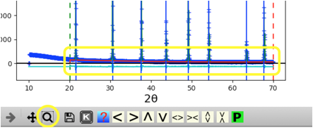
Use the zoom feature (magnifying glass below the plot) to draw a box around the low intensity data.
Looking at the magnified plot (to right), makes it clear that the default number of background terms (3) does not allow enough freedom to fit the curved shape of the background. Increasing the background terms from 3 to 6 will fix this.
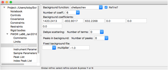
Select the Background tree item and change the number of coefficients to 6, as shown to the right. Then return to the Peak List data tree item and use the Peak Fitting/Peakfit menu item to perform a peak refinement.
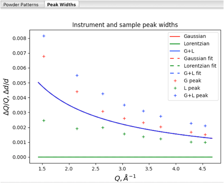
At this point it is instructive to click on the Instrument Parameters data tree item to see a plot of peak widths.
Note that the solid curves here are plots of the profile coefficients from the default instrument parameters (which are unimportant here), but the fits for the individual peaks are shown (in units of Q/\(\Delta\)Q vs Q), with Lorentzian widths (gamma) in green, Gaussian widths (from sigma2) in red. The convolution of Gaussian and Lorentzian (total broadening) for the individual peaks is shown in blue.
When individual peak profile terms are refined (sig2 and/or gam) , those values are used to compute the peak profiles, but when a sig2 or gam value is not refined, these values are generated from the U, V and W terms (for sig2) or X, Y and Y for gam. (Note that Z, which provides for broadening independent of Q, is provided as an option, but is rarely, if ever, appropriate.) It is possible to turn off the computation of sig2 and gam values from the instrumental terms by unselecting the “Gen unvaried widths” menu option, but this is not needed here.
GSAS-II allows X and/or Y to be refined where some (but not all!) gam terms are refined individually, and one may expect to see differing trends in the Lorentzian widths from peak to peak in a sample that contains more than one phase or exhibits anisotropic peak broadening. However, since Gaussian peak widths should arise from instrumental broadening, which should be independent of any sample effects, this mixed mode of fitting is not allowed for refinement of sig2. If any individual peak sig2 values are refined, the U, V and W terms cannot be varied.
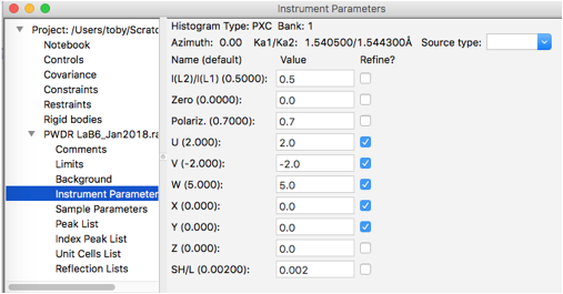
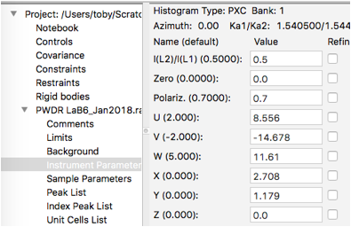
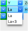
Here we will select to refine the overall profile terms: use Gaussian U, V, & W and Lorentzian X & Y, as shown to the right:
As noted before, we must remove fitting of the sigma2 terms in order to fit the U, V & W terms. If we had any peaks that were not consistent with the width of the others, we might choose to continue to refine their individual Lorentzian profile terms (gam), if that is done, those peaks varied individually would be excluded from the X & Y fitting. Here we will refine U, V, W, X & Y against all peak and will remove all individual peak widths from the fit. To do this, select the Peak List data tree item and remove refinement of sigma & gamma for all peaks by double-clicking on the refine column headers for each and select “N – vary none” so that the table appears as to the right:
Use the Peak Fitting/Peakfit menu item to perform a peak refinement optimizing U, V, W, X & Y. Note that the sigma and gamma values are now computed from U, V, & W and X & Y, respectively.
The difference curve shows only very small deviations, so use of the Instrumental Parameters is very close in quality to the fit with individual peak widths despite being more highly constrained (5 terms vs 16 for the individual case). Note also that the background is also quite well fit now.
So that we can use these profile terms as the starting point for a future refinement, we want to create a file with these terms that we can use for future fits for data from this instrument. However, we do not want to include the sample broadening in this, so before saving the values set the X & Y terms to zero. Note that equivalent to this would have been to have only refined U, V & W, leaving X & Y at their initial zero values and to have refined the individual peak gamma values.
After setting X & Y to 0.0,
save the profile terms to a file by clicking on the
Instrumental Parameters data tree item and use the
Operations/Save Profile menu command. Since different
sets of instrument parameters will be needed for different instruments
and for different configurations (for example, slit settings), it is
wise to include information about the configuration in the file name.
The file extension will be .instparm. Place a copy of this
file where it will be conveniently accessed when reading in data files.
Make a note of this file name, as we will use it in a subsequent
step.
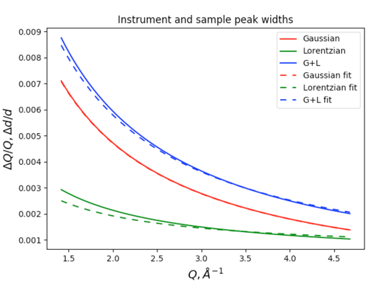
We might want to see how well the U, V & W values reproduce the fits where the sigma2 values were allowed to vary freely. Likewise, comparing widths generated from the X & Y values to the individual gamma values will provide evidence for the presence of a second phase or anisotropic broadening. Also, this provides a place to make the features of the “Instrument and sample peak widths” plot clear.
First, since we have previously set the X & Y values to zero, repeat the previous peak fitting, again using the Peak Fitting/Peakfit menu item to perform a peak refinement that optimizes U, V, W, X & Y. This should provide approximately the same values as seen before.
Next, we stop refining U, V, W, X & Y by clicking on Instrumental Parameters data tree item and turning the refinement flags off for all terms, as seen to the right.
In the Peak List data tree item, turn on the refine flag for all individual peak widths (as was done before.)
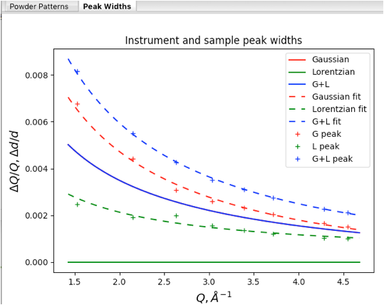
Use the Peak Fitting/Peakfit menu item to perform a peak refinement, again optimizing individual peak widths. Returning to the Instrumental Parameters data tree item provides the plot seen to the right.
This plot uses the following color coding: Lorentzian widths are shown in green, Gaussian widths are in red and their convolution (total broadening) is shown in blue. The plot components are:
Solid curves are the profile terms from the original instrument parameter file (here the CuKa lab data defaults, where the actual values are largely irrelevant here). Note since X, Y & Z are zero, there is only Gaussian broadening and the total broadening is exactly the same as the Gaussian. so the blue curve hides the red one.
Dashed curves: these values are generated by the refined U, V & W and X, Y & Z values. If we had used an instrument parameter file that had been appropriate for the instrument used here, the observation that displayed instrumental broadening here (dashed red curve) is significantly greater than the default values (the solid red curve, which is hidden by the blue solid curve) would be useful information.
Plus signs (for individual peaks) these show the widths for the individual unconstrained peak widths. Note that the Gaussian and Lorentzian fitted widths agree well with the fitted Instrumental parameter curves (dashed lines).
These profile terms are more than adequate for most structural fitting problems, but it should be noted that better values would be preferred to obtain quantitative measurements of microstrain and/or crystallite size. To obtain more accurate terms, start fitting the instrument profile from values determined as was done here in a Rietveld fit. Ideally, use a standard where microstrain and crystallite size effects are known and can be used as fixed values in the calibration. This will allow U, V, & W to be established optimally. As noted before, inclusion of higher angle data would be preferable, as would be a sample with lower angle peaks. With peaks at low Q values, the SH/L can also be refined.
The obvious question will be how well do these parameters fit the data? To test this, we can start a new refinement using the instrumental parameters and see how well they do.
Use the File/New Project menu command to create an
empty project. You can say Yes to the prompt to save the current project
(No would not hurt.) As before, use Import/Powder Data/from
Bruker RAW file to read file LaB6_Jan2018.raw from
the Tutorials CWInstDemo/data directory (downloaded already
from https://advancedphotonsource.github.io/GSAS-II-tutorials/CWInstDemo/data/).
After selecting this file, answer yes to “Is this the file you
want?”
The next dialog to appear is titled, “Choose inst. Param file for LaB6_Jan2018.raw Scan 1 unlike before, we do have profile terms to read, from the file created previously. Select this file as the instrument parameter file and press OK. Note that you may need to change the file filter to see files of type .instparm.
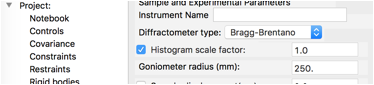
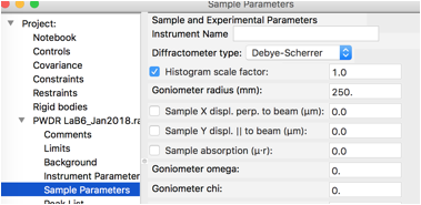
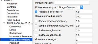
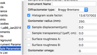
At present, the instrument type is not saved, so go to the Sample Parameters data tree item for the new histogram and change the Diffractometer type from Debye-Scherrer to Bragg-Brentano, as seen to the right.
We will add a phase for LaB\(_6\). Since this is a simple material we will input this by hand rather than trying to import it. Use Data/Add new phase to create a new phase. Enter any name you choose, though LaB6 is a good choice and press OK.
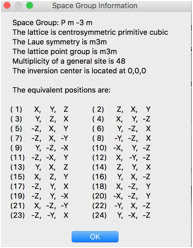
The symmetry and cell need to be edited on the new phase’s General tab. Click on the Space Group Button (which defaults to P1) and enter P m -3 m (note use of spaces to separate symmetry axes – though in this case since this is a standard setting, omitting the spaces works too. The space group symmetry information to the right is displayed, click OK.
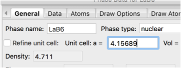
Change the lattice constant (a) from 1.0 to 4.15689 A. (The certified value for SRM 660b)
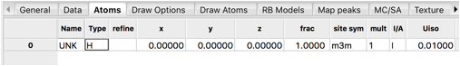
Finally add atoms to the phase by clicking on the Atoms tab. Use the Edit Atoms/Append atom menu item to insert an atom. A new atom is included in the table.
Double-Click on the Type value (H) and which opens a periodic table window. Click on the arrow next to La to bring up a menu of the defined valences. Select La (neutral atoms are usually to be preferred) from that pull-down and the period table window closes. This atom is located at position 0,0,0 so no further editing is needed.
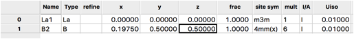
For completeness, add the second atom by using the Edit Atoms/Append atom menu item again to insert an atom. For the second atom, change the type to boron by Double-Clicking on the Type value (H) and selecting B (the only choice) from the pull-down. The coordinates for this atom are 0.1975,0.5,0.5 so the x, y and z values must be edited.
Note that the site multiplicities indicate that the stoichiometry is La\(_1\) B\(_6\), as is expected.
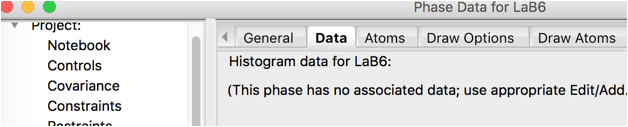
Click on the Data tab for the phase. Note that there are no associated histograms.
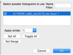
Use the Edit Phase/Add Powder Histogram menu command. Select the one histogram and press OK.
Nothing needs to be changed of the new parameters added here.
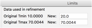
We will first change a few histogram parameters. For data tree item Limits change Tmin to 20 degrees, as was done before.
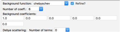
For data tree item Background change the Number of coeff. to 6, as was done before as well. Note that the refinement flag is on by default.
We will not refine any of the Instrument parameters, but we will refine the histogram scale factor (only) on the Sample Parameters. This is also on by default, so it is not necessary to select the Sample Parameters data tree item, but if it is selected it will appear as to the right.
Use the Calculate/Refine menu item to start refinement.The program will prompt requesting a name for the newly-created .gpx file.
The fit is not very good, as seen in closeup to right. Clicking on the histogram’s (PWDR) data tree item and zooming in shows that the reflection ticks are not well aligned with the peaks. This is due to sample displacement.
The position of the sample relative to the scattering circle is never well determined in a Bragg-Brentano instrument, so the sample displacement should always be varied. Click on Sample Parameters and turn on refinement of Sample displacement.
Use the Calculate/Refine menu item to start another refinement. Significant improvement is seen and even more if Calculate/Refine is used a second time.
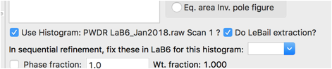
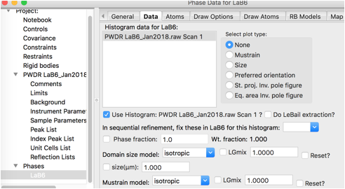
Part of the problem in the fit is that the intensities are not well fit by the crystallographic model. Rather than fitting the few free structural parameters (x for B and Uiso values), we will treat the intensities as arbitrary, using Le Bail fitting. This is done by clicking on the Phase tree item and the Data tab and setting the do LeBail extraction flag.
Use the Calculate/Refine menu item to start another refinement. A warning message that “Steepest Descents dominates” is shown because a high degree of parameter correlation occurs as the reflection intensities change. The fit does not improve very much if Calculate/Refine is used a second time, but the warning goes away.
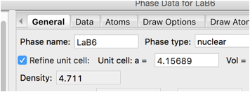
While this should not be needed for a standard, it is clear by looking at the plots that peaks are still not quite lined up. In a less dense sample it might be reasonable to refine the sample transparency, but for highly absorbing LaB\(_6\), that is not a reasonable parameter. A better fit requires refining the lattice. On the Phase/General tab press the Refine unit cell control.
Use the Calculate/Refine menu item to start another refinement and the positioning of the peaks improves significantly.
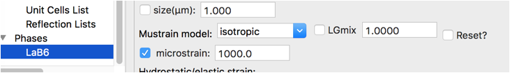
The remaining major problem is that we have not treated the sample broadening and LaB\(_6\) does have some microstrain. That can be refined with the Phase/Data tab with the microstrain control.
Use the Calculate/Refine menu item to start another refinement. A second refinement cycle brings the Rw to circa 5.8%, with the fit improving dramatically.
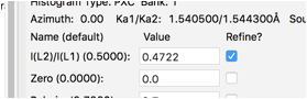
For these data, it appears the ratio of K\(\alpha_1\) and K\(\alpha_2\) is not exactly the theoretical value of 0.5. This can happen due to a slight misalignment in the monochromator setting. Allowing this to shift slightly by including this in the fit brings the Rw to circa 4.9%.
The fit is quite good without fitting the instrumental profile terms:
The quality of the profile parameters we previously fit can be demonstrated by turning off refinement of the microstrain term and refining the U, V, W and X & Y terms. This produces a small improvement in the fit (expected as 1 fitting parameter as been replaced by 5), but the actual changes are very small, as noted by the Instrument Parameter terms plot:
In this section we fit a pattern with a wider range of data. This proceeds quite simply.
Restart GSAS-II or use the File/New Project to create a new empty project.
Use Import/Powder Data/from GSAS powder data file to
read file NIST660CBI.gsas from the Tutorials
CWInstDemo/data directory (download from https://advancedphotonsource.github.io/GSAS-II-tutorials/CWInstDemo/data/).
After selecting this file, answer yes to “Is this the file you want?”.
As before, use Cancel to select the default CuKa lab data instrument
parameters.
Since the background for these data is quite curved at lower angles, reducing the angular range to be fit will require fewer background terms. Select Limits in the data tree and then set Tmin to 20. Then select Background in the tree and change the number of background parameters to 8.
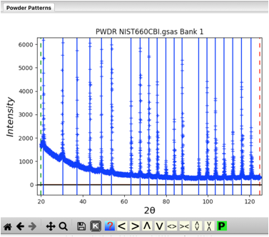
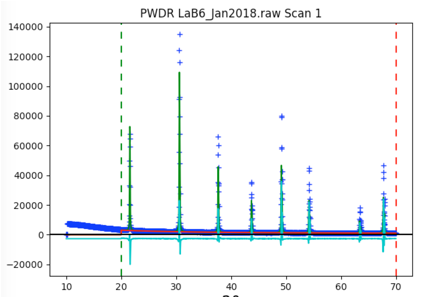
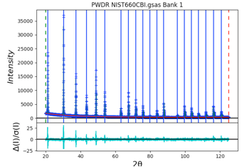
Select Peak List from the data tree to allow adding peaks. Zooming in on the lower portion of the pattern makes it easier to see all the peaks. Be sure to click on magnification icon a second time to turn off zoom mode. Then click on a point for each of the 20 peaks in the pattern. You should have a plot that looks like this:
As the peaks are initially added to the table, the refine flag is set for the peak intensity. Fit the individual peak intensities by using the Peak Fitting/Peakfit menu command. Provide a file name and the Rwp drops to ~40% with a reasonable background level, but as before, poor initial (unrefined) peak shapes.
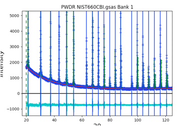
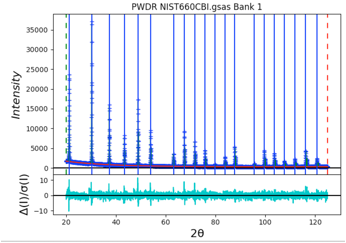
Select the Instrument Parameter tree item, select the refinement flags for U, V, W and SH/L, then select the Peak List tree entry again and use the Peak Fitting/Peakfit menu command. The fit improves a bit, but since the peak positions have not been refined, a good fit is not expected. Click on the refine column heading (to the immediate right of the peak positions), then select “Y” and “vary all” and again use the Peak Fitting/Peakfit menu command. Add refinement of the gamma values by clicking on that column heading. The fit improves significantly with an Rwp value of ~8%. The fit shows very small difference plot. However, pressing the “w” key in the plot window changes the plot appearance to that on the right where it can be seen that the fit at low angle is significantly worse than at high angle. This suggests that low-angle asymmetry correction is not being fit well and is stuck in a locak minimum.
To improve this, we can force the SH/L value to be larger. Instead of the local minimum that was found with SH/L of ~0.003, we can select the Instrument Parameter tree item and set SH/L to a larger value, say 0.03. Then select the Peak List tree entry again and use the Peak Fitting/Peakfit menu command. The Rwp improves somewhat, to circa 5%, but now the difference plot is greatly improved at low angle with SH/L increasing to 0.063.
Select the Instrument Parameter tree entry and then use the Operations/Save Profile… menu command to write a file. Note that in this case, the X & Y values were never refined, so they do not need to be reset manually before the file is saved. Again, the file produced here can be used to determine the instrumental profile terms for future refinements and these terms do not need to be refined . The plot shown when the Instrument Parameter tree entry is selected compares the mostly meaningless default starting profile terms (as solid lines) to the fit results (as dashed lines and plus signs for individual peaks). Using Operations/Load Profile… will set the initial (default) instrumental values to the current refined parameters, which makes for a simpler plot as the dashed and solid-line curves are now superimposed.