Tutorial: Preparing a Full CIF

·     Exercise files are found here. The data files are taken from the conclusion of the “Combined X-ray/neutron refinement – PbSO₄” tutorial.

Background

Crystallography has had a long tradition where experimental data as well as results were reported numerically, so that results could be verified independently as well as utilized. In the past two decades the field has set the standard for data science compared to almost all other areas of physical and biological science through the development of the Crystallographic Information Framework (CIF) which defines a universal format for the reporting of nearly all aspects of a crystallographic fit. This is particularly true for Rietveld fits, where the pdCIF subset of CIF has been developed to capture the observed and computed patterns as well as reflection tables and coordinates as well as interatomic distances and angles.

 

Within GSAS-II, a CIF for a phase are available as “quick” coordinate-only file, which provides atom coordinates and displacement parameters, but no uncertainties or other supporting information from the refinement. This is indeed easy with a single menu command. Likewise, a CIF containing only a dataset without phase information can be easily created from the Export menu, but the real power of CIF comes after a project has been completed. Using the “Entire project as…” a “Full CIF” menu command in the Export menu, all results can be reported in a machine and human readable. There are a few steps in generating a full project CIF. This tutorial goes through them and explains what is being done and why.

 

A bit of background on CIF: The format allows a label (a CIF data item, such as _cell_length_a or _publ_author_name) to be associated with either a single value or a column in a table. A collection of data items is placed in a block. For a single-crystal structure, a block will usually contain the coordinates for a phase and the structure factors (experimental data and the matching simulated values) as well as supporting information and derived results. With multiple temperatures, a block would be needed for each setting because, for example, only one set of unit cell dimensions and coordinates can be defined in a block. With powder diffraction, if a single dataset (histogram) is used and only one phase is present, a single block can be used. If either more than one phase is present, or more than one histogram is used, multiple blocks are required. GSAS-II will create single-block CIFs when possible, but otherwise will create a block for the overall refinement plus a block for each histogram and a block for each phase. Referencing information between different blocks requires that each block be labeled with a unique name. These block labels are assembled from a number of fields supplied by the user and a timestamp when the file is created.

 

A tremendous amount of information can be placed into a CIF file. No one is likely to specify all of the field in the IUCr-supplied template, which itself does not include all data items defined in CIF. Some information can be supplied by GSAS-II from what is defined inside a project, data such as symmetry and lattice parameters, but other information, for example synthesis conditions or sample color, must be supplied by the user. This could be done with a simple text editor once the file is created, but the problem that arises from that approach is that it is common that after one has produced the “final” refinement, another idea occurs for a slightly better fit. The approach used in GSAS-II is that as the CIF is generated, copies of template files are made that contain all the user-supplied information. Thus, the CIF can be recreated from the updated project without having to repeat all the work in supplying that information. Also, by saving template files that have setting information that will be common amongst multiple projects (for example, diffraction instrumentation descriptions) these files can be reused, avoiding repetitive tasks. 

Prerequisite

Before beginning this tutorial, either complete the refinement in the “Combined X-ray/neutron refinement – PbSO₄” tutorial or download the GSAS-II project file provided here, which provides a two histogram, one phase refinement.

 

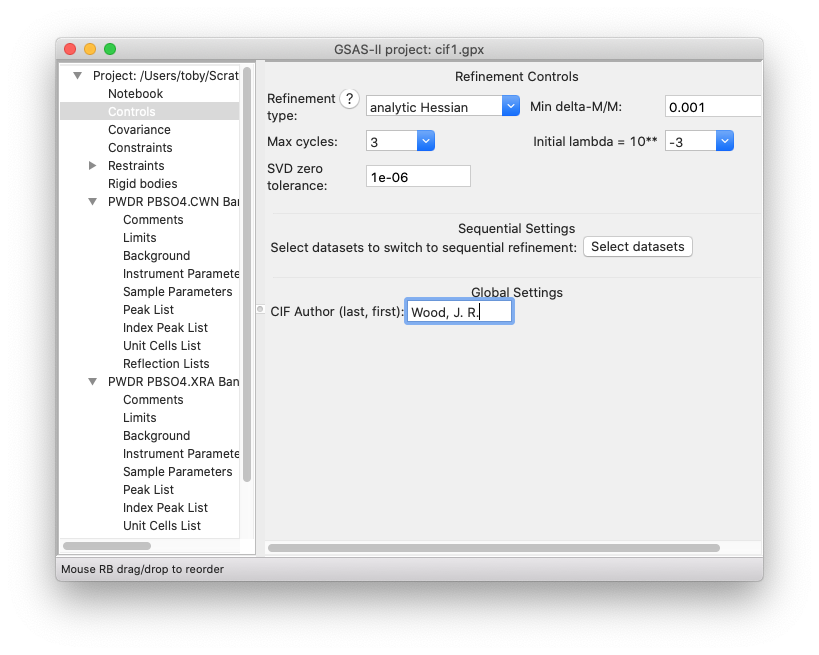
Part 1. Enter a name for the author of the CIF file.

 

·     Select the Controls entry on the data tree and enter the name for the main author for the project and CIF.

 

 

Part 2: Start the export process

 

·     Using the Export menu, select the “Entire project as” menu item and the “Full CIF” submenu option.

 

 

This opens a dialog (exact appearance will depend on the operating system you are using) where you can select a name for the file to be created.

 

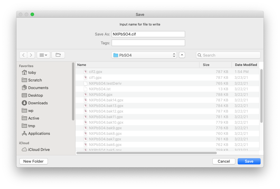
·     Enter a name for the file if you wish to override the default name and press Save. If that file exists, you will need to agree to overwrite it or to select a new name.

 

Part 3: Select instrument name(s)

 

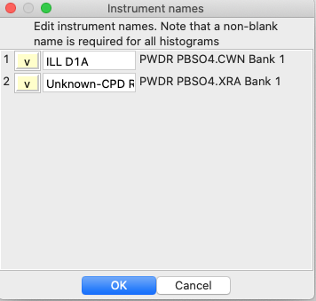
Before a CIF can be created, each histogram must have associated with it an instrument name. Note that the instrument name appears in the Sample Parameters tree entry for each histogram. If any instrument does not have a name, the dialog below is displayed.

 

 

 

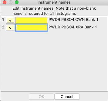
Ideally the instrument name will be unique, so the combination of the name and a timestamp will create an identifier that is unlikely to be repeated. The instrument name should also allow the data source to be identified should there be several similar instruments within an institution, but the details for naming are left as a local decision. Inclusion of an institution name is a good idea, so an ideal name might be “Univ. of Mars, Curiosity II”. While in this case the two histograms are from different instruments, the down arrow (Ú) button will copy the entered name to all fields below, simplifying the data entry task, when appropriate.

 

·     Enter names for each instrument and then press OK.

 

Part 4: Bond distance/Angle criteria

 

One significant part of a CIF is the computation of bond distances and angles. For this there is a set of atomic radii for each phase along with a tolerance factor. When the CIF creation is initially invoked, the dialog below is shown for each phase:

 

 

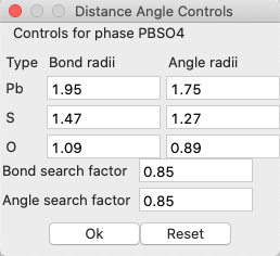
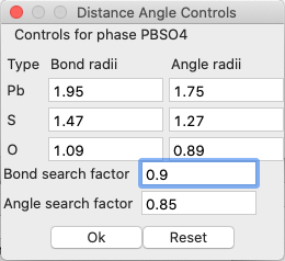
This dialog will not be shown again, unless invoked manually. To explain what these numbers mean, distances between Pb and O atoms will be reported when their interatomic distance is less than or equal to (1.95+1.09)*0.85 Å (=2.584 Å) and O-Pb-X or X-O-Pb angles will be reported if the Pb-O distance is less than or equal to (1.75+0.89)*0.85 Å (=2.244 Å) and the O-X or Pb-X is within the requirement for that pair of atoms as well (in this case X could be O, Pb or S).

 

·     At this point no changes are needed, so simply press OK.

 

Part 5. Conditions warning

 

Note that when a histogram is created in GSAS-II, unless pressure and temperature values are reported in the metadata in a standardized fashion (this is uncommon), the sample temperature defaults to 300 K and the ambient pressure to 0.1 MPa. It is likely that these values do not describe the actual data collection conditions. Since they will be included in the CIF, they should be updated with more appropriate values.

 

 

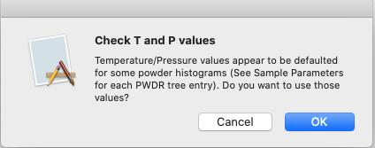
The warning above will be shown every time the code for CIF generation code is initiated, unless the sample temperature has been set to a value other than 300 K for each histogram. If indeed the histogram temperature/pressure values are correct, this warning may be ignored. Note that the Command/“Copy Selected” menu command may be useful to change a value in multiple histograms in one operation.

 

·     Press Cancel to stop the export

 

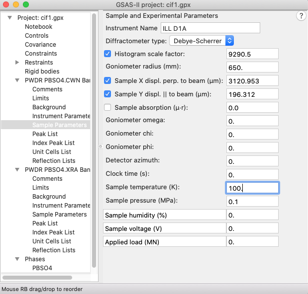
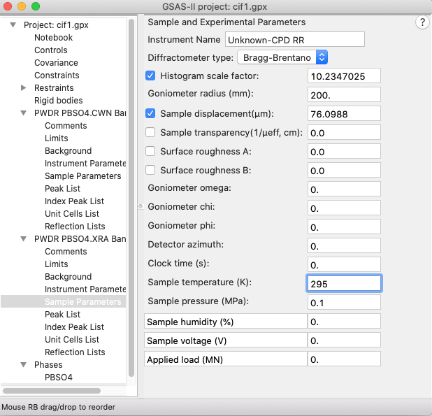
In this case it is of particular importance to note the data collection temperatures. The neutron dataset was collected at cryogenic temperatures, while the x-ray data were collected under ambient conditions.

 

·     Change the temperature values in each histogram, as shown below. Note that ideally, temperature and pressure values will be available to GSAS-II in a data file’s metadata and will be set in the Sample Parameters automatically, but this is seldom the case.

 

 

 

 

Part 6. Restart the export process

 

·     As before, use the Export menu and select the “Entire project as” menu item and the “Full CIF” submenu option. If you use the same file name as in Part 2, you will likely need to say yes to overwrite the file.

 

Note that the windows opened previously in steps 3-5 will not occur again, since the requested information has been provided.

 

Part 7. Specifying CIF Contents.

 

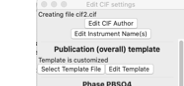
Once the previous steps have been performed, a window such as the one below is shown. Note that the “Edit CIF Author” button opens a dialog window, where the information supplied in Part 1 can be changed. The “Edit Instrument Name(s)” button reopens the window shown in Part 3.

 

 

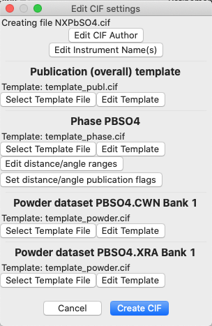
Note that for every other section of the window, there is are a pair of buttons labeled “Select Template File” and “Edit Template.” A default template file is selected initially, and information can be included in that template with the “Edit Template” button, as will be shown below. Note that there are four types of template files for (1) overall information; (2) phase information; (3) powder diffraction data and instrumentation details; and (4) single-crystal diffraction data and instrumentation details. Note that data items that are set by GSAS-II directly (for example, lattice parameters and space group information for a phase) are not included in the template.

 

The information you specify to place in a template is included in the GSAS-II project (.gpx) file so that if you perform a new refinement, all of the template edits you have made are used automatically when a new CIF is created.

 

As you are editing each template, you can save that information in a file. There are two reasons for doing this. One is that by saving the information as a file you potentially create a customized template file. Use of this file in the future for a different project can save you considerable time, as an example, when documenting a diffractometer. Also, if a file is saved, instead of keeping all of the template contents in the .gpx file, only the name of the template file is saved, reducing the project file size slightly. (The default template files range from 1K to 4K bytes in size, so this not usually very significant savings.) Once a customized template file has been created, use the “Select Template File” button to select it in place of the default.

 

·     Edit the Publication template by pressing the “Edit Template” button closest to the top of the window [just below the “Publication (overall) template” heading] a window similar to the one below is created.

 

 

A few notes on the arrangement of this window, which is a bit easier to use if manually resized, as below.

 

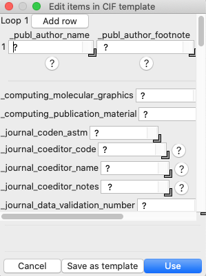
Note that this contains three CIF items, _publ_author_name, _publ_author_footnote and _publ_author_address, in a table (loop_). Note the “Add row” button to the upper left which allows additional rows to be added to the table. The remainder of this template is a series of CIF items that accept a single value. Most CIF items are tagged with a help button, marked with a question mark. That indicates that that CIF item is defined in a CIF dictionary. The definition can be looked up by pressing that help button or by allowing the mouse to stay stationary on a CIF item name for a few seconds which causes the definition text to appear as a tool tip, as below,

 

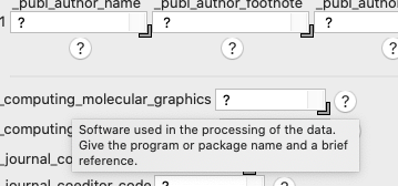
or clicking on the button displays the same information at the bottom of the window, as below.

 

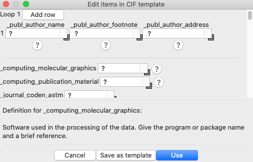
Note that each text entry box has a small right-angle bracket (looking a bit like an inverted L) at the lower right corner. This can be used to resize the text entry box to allow viewing a longer line of text and/or several lines of text.

 

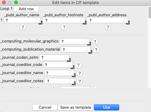
·     Press the “Add row” button to create entries for a second author.

·     Enlarge the width of either of the _publ_author_name entry boxes as well as the height and width of the _publ_author_address item to accommodate more text.

·     Add text to describe authorship, such as what has been done below (authorship of the original Anglesite, aka PbSO₄, crystal structure). Note that as is described in the CIF definition, author names are supplied as last name, first name.

 

 

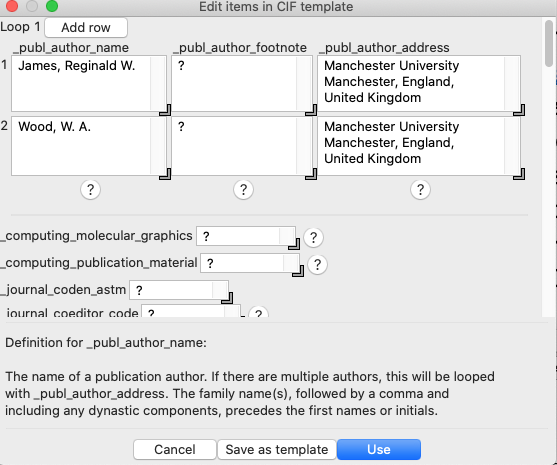
·     After completing all appropriate CIF items that would be appropriate for this work, press the “Use” button to close the window, saving the entries into the project file.

 

Note that the window contents changes to indicate that the template information is no longer from a file.

 

Part 8. Edit Phase Information including Distances and Angles.

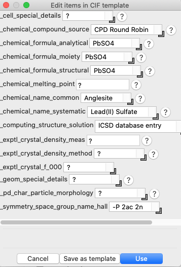
The phase template contains a relatively small number of items that can document information about a phase, as shown below. If one produced several projects all using the same sample, it might make sense to produce a template file that might be used for that sample in all projects.

 

·     Press the “Edit Template” button in the Phase section of the “Edit CIF settings” window and the window below appears. Enter any information desired. Press “Use” when done.

 

 

 

 

·     Press the “Set distance/angle publication flag” and the window below appears.

 

 

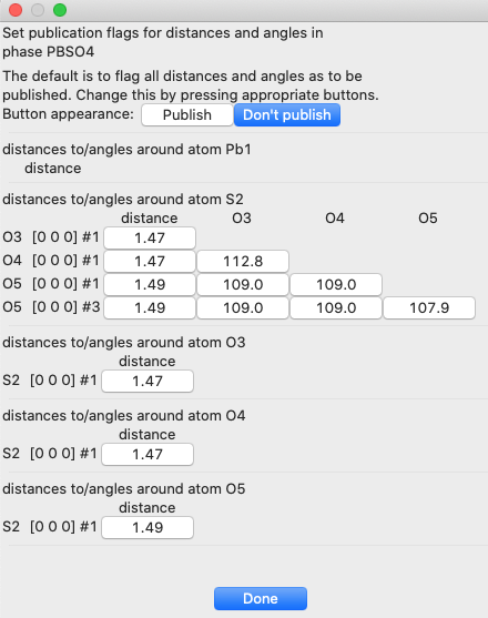
This shows the interatomic distances and angles that that occur within the radii specified above. Note that the Pb radius is too small to pick up the coordination of that atom, so we should change that:

 

·     Press the “Done” button to close this window

·     Press the “Edit distance/angle ranges” button to bring up the screen below. Change the bond search factor from 0.85 to 0.9 to increase the search range, as below.

 

 

·     Press the “Set distance/angle publication flag” and note the additional distances (but not angles) in the window below.

 

 

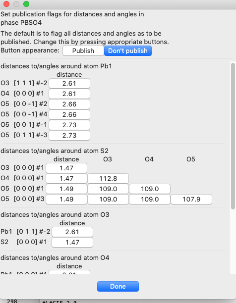
Note that to obtain the angles around the Pb and O atoms, the values in the right-hand column and/or the angle search factor range must also be extended.

 

Every bond and angle that is listed on the window will be placed in the CIF when written. Note that while distances and angles are shown in the window without uncertainties, if the atom positions have been varied, the values with their uncertainties will be placed in the CIF (in standard crystallographic notation). Also note that in the CIF each distance has an associated _geom_bond_publ_flag value (for angles, _geom_angle_publ_flag). The value for this can be “yes” or “no” and a “yes” value indicates that the value should be placed in a table of bond distances/angles, if generated from the CIF. By default, this flag defaults to “yes” but this can be changed by clicking on the distance or angle button.

 

Part 9. Create a Customized Template File.

 

For this particular project, since these were data distributed from a round-robin study many years ago, relatively little is documented on the instruments, but as a useful exercise, I recommend opening documenting an instrument that you use frequently (or twist the arm of the instrument scientist at your favorite facility to do so.) 

 

·     Press the “Edit Template” button for either histogram and define as many of the appropriate fields as are appropriate.

 

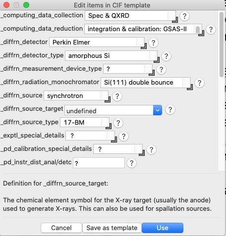
·     Press the “Save as template” button and save the file with a name and location that will make this readily available for future use.

 

Note that the next time that “Export… project… to CIF” is used, this template can be used by pressing the “Select Template File” button for that histogram and by doing this all of the information specified previously can be used without additional data entry effort. 

 

Part 10. Create the CIF

 

·     Pressing the “Create CIF” button will cause the CIF to be written.

 

Depending on the number and size of histograms, this can be a fairly large file as it contains observed and computed patterns for each, as well as a reflection table, plus unit cell parameters, symmetry information, coordinates and bond distances and angles for each phase.

 

Note that if the refinement information is changed, for example by introducing a new variable, changing the background model etc. all that need be done to create a CIF with updated information will be to select the “Entire project as” menu item and the “Full CIF” submenu option from the Export menu and then press the “Create CIF” button again. All information generated by GSAS-II will be updated and previously entered will be retained and placed in the new file.