Fitting the
Starting Background using Fixed Points
Introduction:
There are times when it can be difficult to establish a good initial model for the background in a Rietveld fit. The authors of GSAS-II feel that background models should always be refined in the final stages of refinement (on occasion when background levels interact highly with atomic displacement parameters, one may need to fix one or the other), but in the initial stages of the fit, it can be helpful to force the initial background fitting to follow a curve supplied by the user. This tutorial shows how to do this.
For this example, we will fit data from 11-BM that has a fairly large broad background peak.
Step 1. Load the
diffraction data
Import the data using Import/Powder Data/from GSAS powder data file. Change the directory to the location of this exercise (FitBkg/data – yours might be different). Switch the input file type to use zip archives (.zip). Select file OH_00.zip.
This will present a file browser where the data file, OH_00.fxye can be selected.
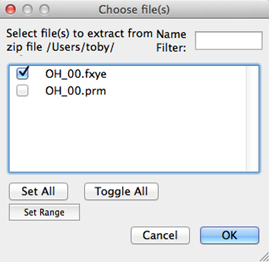
A prompt is presented where the header of the file is shown. Press Yes. The instrument parameter file will be read automatically from the .zip file for you.
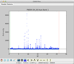
The initial plot of the data does not show much of a background,
But if this plot is magnified, it becomes clear that there are three effects taking place.
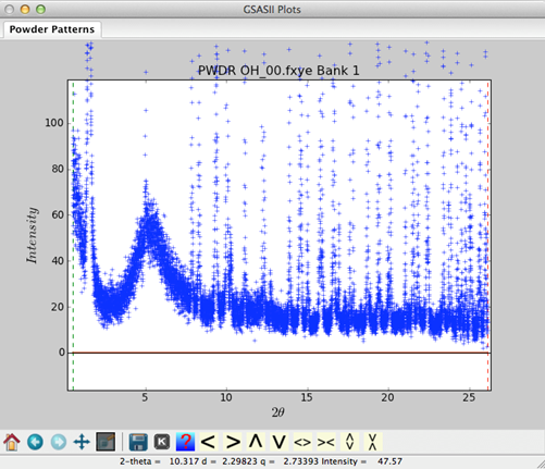
At low angles (below 3° 2θ), there is a
strong fall-off in background (this is due to air scattering & small angle
scattering by the sample); between 3° and 10° 2θ there is a broad feature (from kapton
used to hold the sample) and finally beyond 10° the background is relatively flat. There may be some minor ripple
in this, but this is better explored late in the refinement by looking at the
difference curve.
Step 2. Define fixed
points
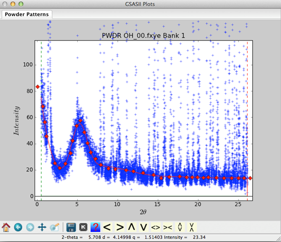
To fit this, we will initially define points where we think the
background should be using the mouse (be sure that the plot zoom &
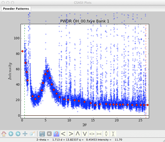
reposition buttons are not selected). Select the Background tree item (under PWDR OH_00…) and from the menu select Fixed Points/Add (Add will then have a bullet selection). Click the mouse at
locations across the pattern to define where the background should go. Select
at least two points for every term that you will want to fit. It is a good idea
to have a point below the lower data limit and one above the upper data limit,
as these will be used in extrapolation.
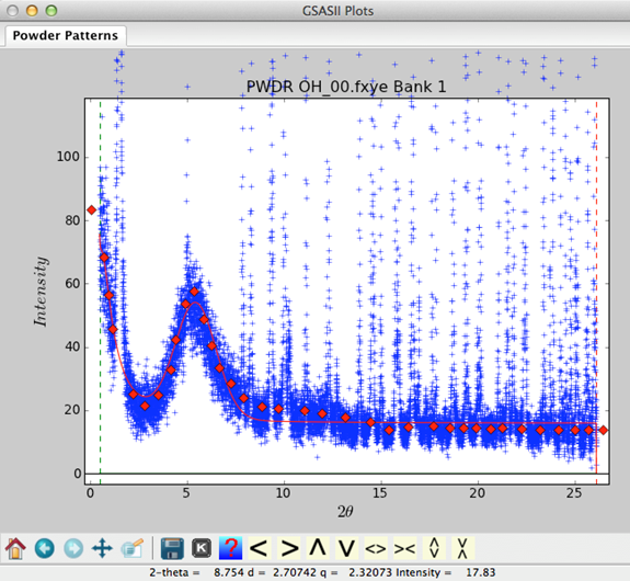
Note that any unwanted points can be deleted by selecting Fixed Points/Delete and then by clicking
on the points. Alternately, points can be repositioned by selecting Fixed Points/Move and then dragging the
points to new locations. The bullet selection on the menu will indicate which
of these is active. When done you should have a plot that looks something like
this:
Step 3. Fit the
background
At this point is becomes possible to fit different background models to the points to see how they do. Change the function, the number of terms, refinement flag(s) and then press Fixed Points/Fit Background menu item. Use of 12 Chebyschev terms gives an OK fit, as shown below, but does have some extraneous “blips”:
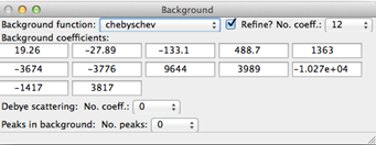
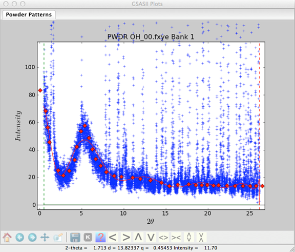
Adding more terms does improve the fit.
Step 4. Add a background
peak
A better choice is to reduce the number of terms and add a background peak to match the feature centered around 5.3 degrees. Initially set the intensity and peak width (but not the position) to be refined.
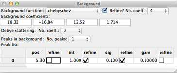
The initial fit is not that good,
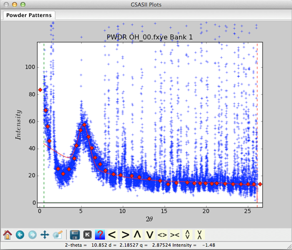
but increasing the number of terms to 8 and refining the peak position as well does give a good fit:
Step 5. Try other models
One of the nice features of this approach is that we can try out different functions and see how well they do.
The Q^-2 power series does a very nice job for the low-angle portion of the pattern with only 4 terms, but does not do very good job at higher angle, even if more terms are added:

While the log-interpolate function does well with only 6 background terms:


Step 6. What to do next
The background points that have been defined are saved in the GSAS-II project (.gpx) file and will appear when the Background menu item is selected. They will not affect the refinement in any way. Nonetheless, you may wish to delete them so they do not appear on the background plot. To do this, use the Fixed Points/Clear menu item. You’ll need to Save/Save as… the project file if you want to retain this new background model for further use.
With the one added background peak, and either the Chebyschev function with 8 terms or the log-interpolate function with 6 terms, one has a good background model to start the fitting. Turning off the refine flags in the early stages of the refinements will simplify the computations and ensure the model stays in a good place, but remember to turn the flags back on in the final stages of fitting.