Create a Background Starting Point with Auto Background

*  A file for this exercise is found here

 

In this exercise the “auto-background” feature of GSAS-II, based on the pybaselines Python project, will be used to establish the background for a histogram as a fitted function. Once that is done, the background parameters used for the first histogram are used to compute a background for the other four files in the project. 

Step 1: Read data into a new project

Start GSAS-II or use the File/New Project menu item to create a new, empty GSAS-II project.

 

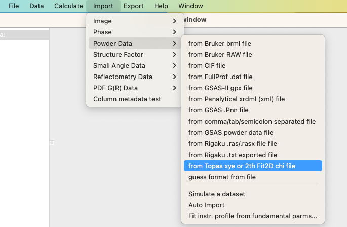
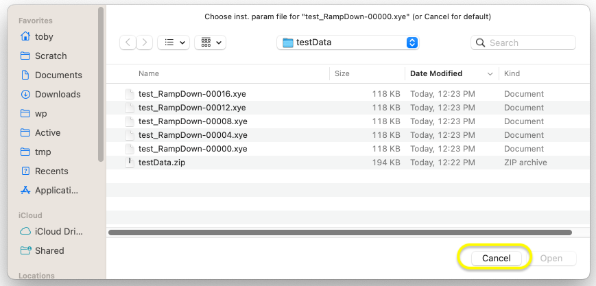
Use the Import/Powder Data/from Topas xye… menu command to open a file browser:

 

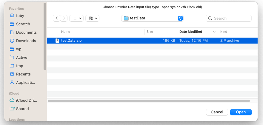
In that browse select the .zip file containing the supplied set of data files, testData.zip, for this exercise.

 

 

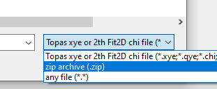
Note that on Windows the file type needs to be changed to “zip archive” to see this file:

 

Once the file is selected and Open is pressed, a selector is offered with five files:

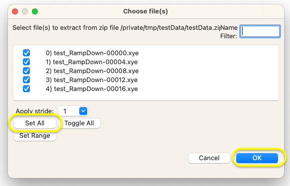
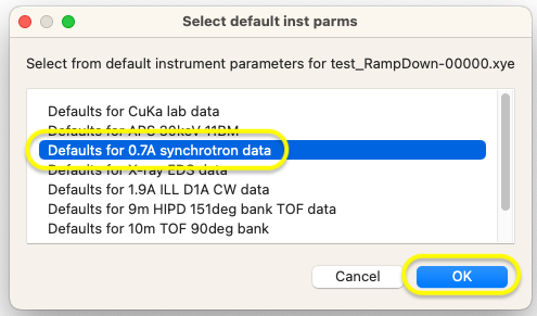
Press “Set All” to select all five files and then “Ok” to to import them into GSAS-II. The program will then ask for an instrument parameter file for these patterns. Since we do not have one, we will select “Cancel” to obtain a default set.

At this point a set of choices are offered. For the purposes of this exercise, it does not matter which option is selected, but the closest option is likely that of 0.7Å synchrotron. If a Rietveld fit would be performed, the wavelength would need to be updated in each histogram. Press “OK” to continue.

 

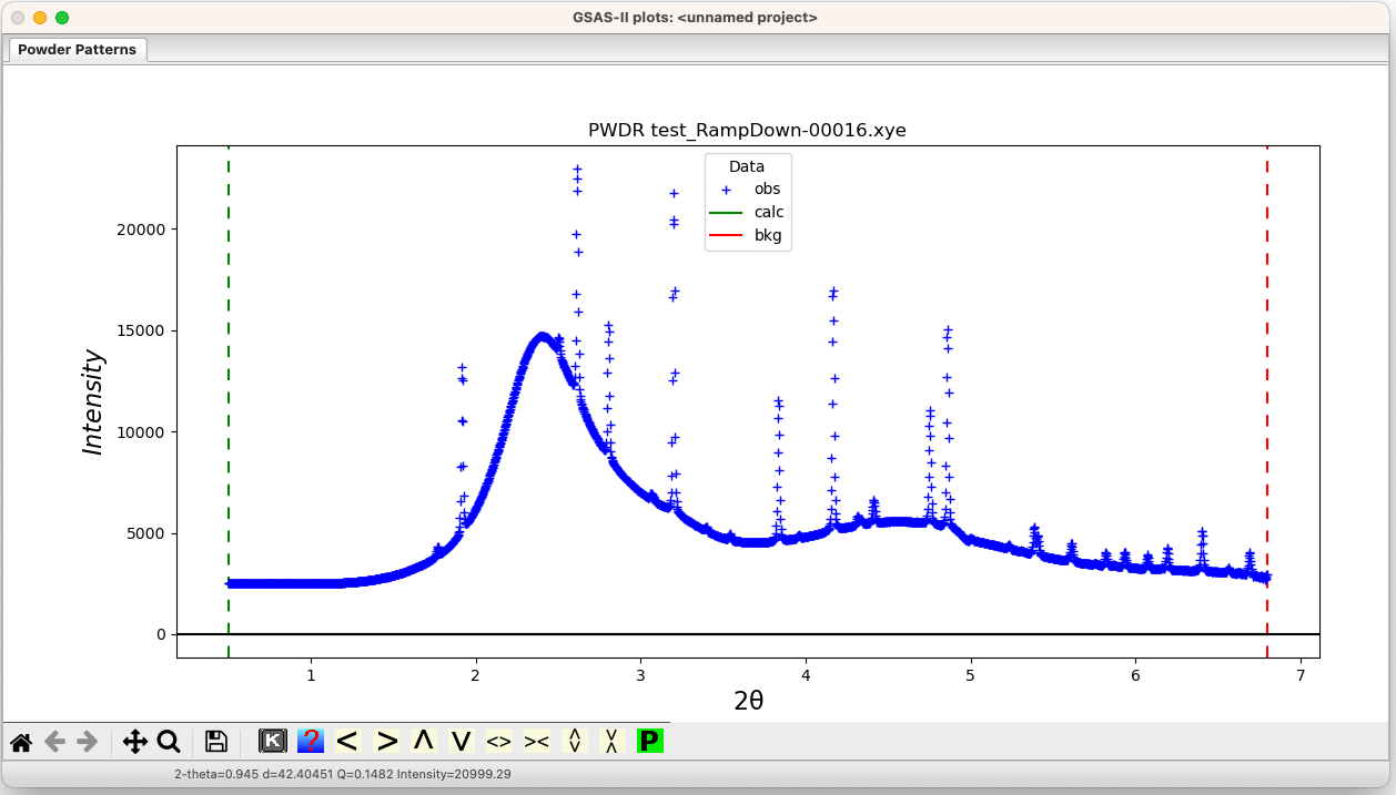
At this point, five histograms will be read into GSAS-II that appears similar to what is below. Note the very pronounced background (probably >100x more integrated background counts than in the Bragg peaks) generated from a furnace.

 

 

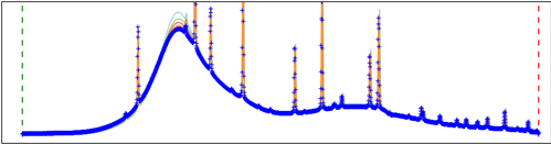
If the “m” (for multiplot) key is pressed in the plot window, it becomes clear that the background is not constant from run to run and must be corrected individually, but the general shape for the background is very similar.

 

 

 

Step 2: Compute the Automatic Background

Select the Background tree entry for one of the histograms. Any will do for this, but I used the first. If needed, position/resize the two GSAS-II windows so that most of the plot window and the main GSAS-II window are both visible. Then press the “Compute auto background” button. The main window will appear as below:

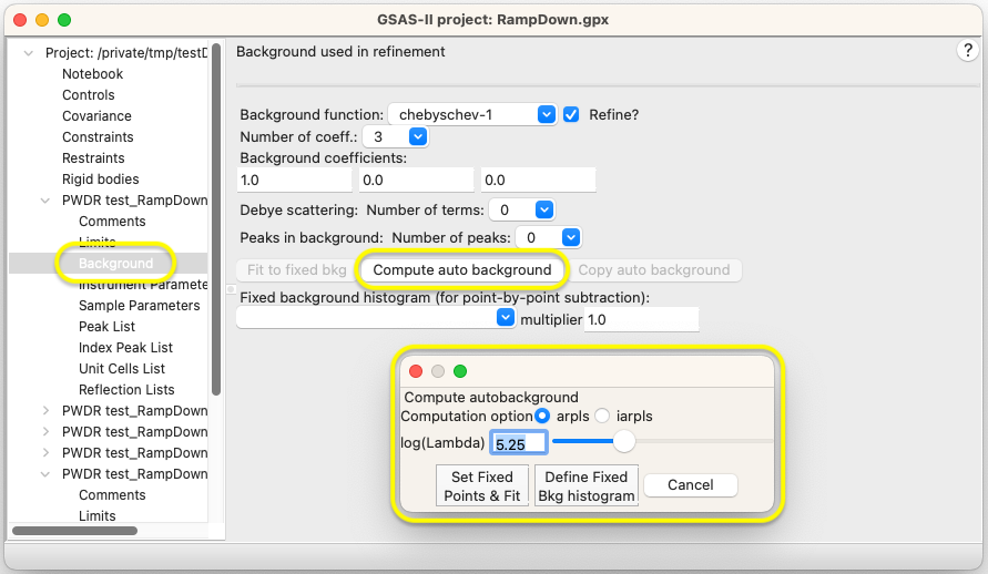
Note that the pop-up window labelled “Compute autobackground” has shifted slightly. The “auto-background” computation is performed immediately and is shown in the plot window, where the blue “plus” signs indicate data and the red line is the computed background:

 

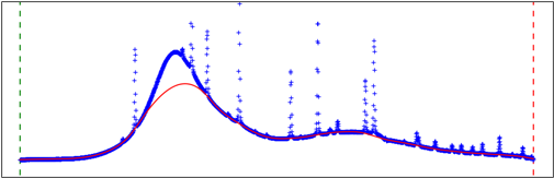
The “lambda” parameter used in the “Whittaker” functions in pybaselines determines how “smooth” the background computation will be, which is in turn influenced by the number of points in the pattern. The larger “Lambda” the smoother the background function. Moving the slider to smaller values, or typing a number around 3.5 into the log(lambda) box allows a good fit for the background:

 

 

 

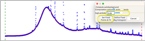
Press the “Set Fixed Points & Fit” button. This places ~100 Fixed Background points along the computed background and then refines that background parameters to best-fit the background function to the Fixed Background points. Since there are only three background terms to fit, the fitted background (the red line) is not very good.

 

 

Step 3: Fit the Background Function to the Fitted Background Points

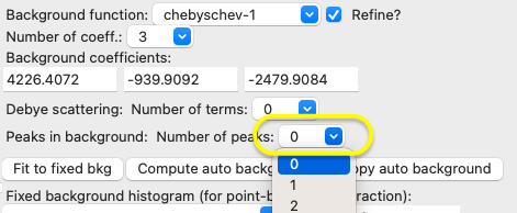
By fitting a background function to the computed background, we will later have the option to refine that background to optimize it. This is the preferred way the treat background for Rietveld fitting. We could try to fit this background by introduce more and more terms into the Chebyschev polynomial to best duplicate the curves in the background, but we will do much better to introduce several broad peaks into the fitting. Moving the mouse in over the pattern, it becomes clear the most significant peak is at ~2.4 degrees. We change the number of background peaks by clicking on that: and then select “1” in the drop-down menu:

 

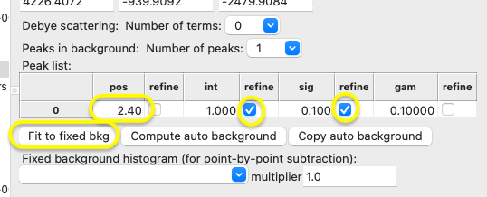
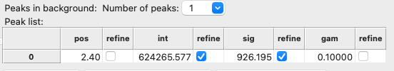
A peak is added to the table, as below. Edit the position to 2.4 degrees and set the intensity and sigma (Gaussian width) refinement flags and then press the “Fit to fixed bkg” button.

 

 

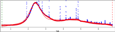
Then press the “Compute auto background” button (this is identical in function to the Fixed Points/Fit background menu command). The fit will be considerably improved, though less than adequate, and main window will be updated, as below:

 

 

 

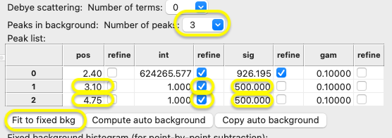
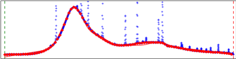
We can see that there is a second peak as a shoulder at ~3 degrees and another peak in the range of 4.5 to 4.8 degrees. Change the number of peaks to three, and add position the new peaks at 3.1 and 4.75 degrees. Refine the intensities, but start the width as something similar to the width of the first peak (I used 500, which is ~half that width.) Finally, press the “Compute auto background” button again.

 

 

The fit improves significantly, but we can do even better.

 

 

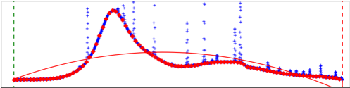
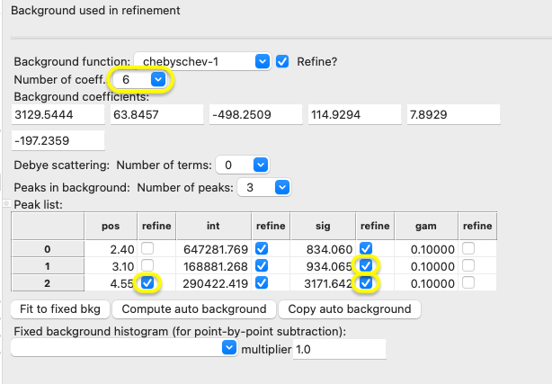
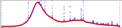
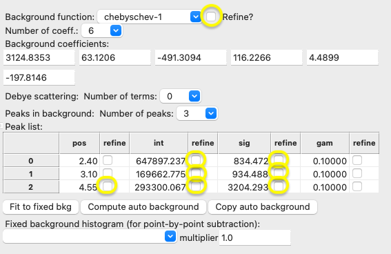
First, we add the widths for the second and third peaks to the fit and press the “Compute auto background.” Then, increase the number of Chebyschev terms to six and refine the position of the third peak. After fitting the results appear as below. This is certainly a good starting point for a refinement:

 

 

 

Step 4: Repeat AutoFit on Remaining Patterns

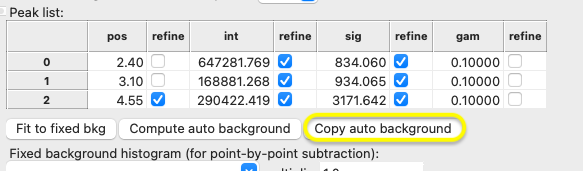
We can use the auto-background with the same log(Lambda) value, generate Fixed Background points and then fit with the same background terms on additional patterns using the “Copy auto background” button.

 

 

When this is pressed, a selection window is opened to choose the additional histograms:

 

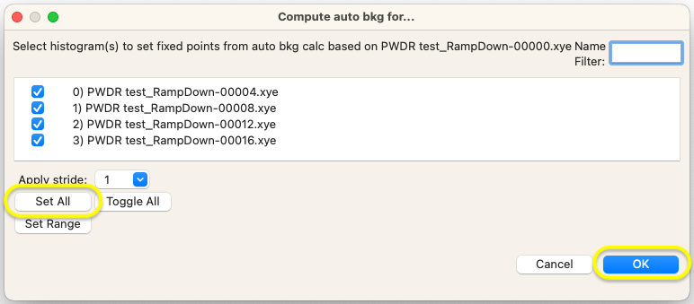
Press “Set All” to select all other histograms. When “OK” is pressed, the auto-background and fitting process is repeated on all patterns. Clicking on the Background data tree item for each histogram shows that Fixed Background points have been assigned for all patterns and the background is well fit.

 

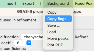
Finally, since this background is a good starting point for refinements, in one histogram turn off all the background refinement flags:

 

and use the Background/Copy flags menu item to use these refinement flag settings for all histograms.

 

Alternate approach: Define a Background Histogram

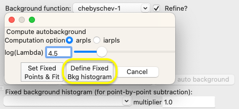
An alternate approach to using the auto-background curve is to use that background as a “Fixed background histogram.” This defines a new histogram for the pattern which is subtracted point by point from the measured pattern. The Fixed background histogram is designed for use where background is measured and only a multiplier is refined, so this is not the preferred choice for Rietveld refinements, but for a highly irregular background that is not easily fit, this might be the best choice. To do this, in Step 2, rather than pressing the “Set Fixed Points & Fit” button, press the “Define Fixed Bkg histogram” button.

 

 

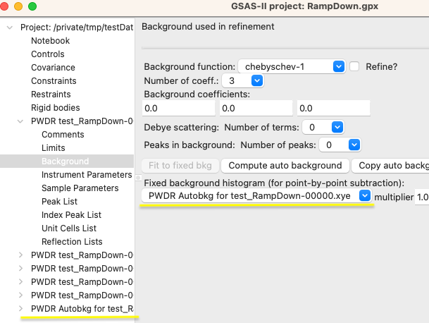
When this is done, a new histogram is defined and set as the Fixed background histogram. The background terms used for fitting are set to zeros and refinement flags are turned off:

 

 

Note that this should only be done once, as a new Fixed background histogram is created each time the “Set Fixed Points & Fit” button is used.

 

If the “Copy auto background” button is used, as in Step 4, a Fixed background histogram is created for all selected histograms. Again this should also not be repeated as a new Fixed background histogram is created for each selected histogram each time the “Copy auto background” button is used.